Geographic data manipulation

Geographic data

Outline for this part: - Vector data - Raster data - CRS - Vector / Raster interactions - Recap Exercise

import pandas as pd
import shapely as sp
import contextily as ctx
import geopandas as gpd
import matplotlib.pyplot as plt
import numpy as np
import rasterio
import rasterio.plot
import requests

import requests
import tempfile

Vector data

Introduction

# "https://datacatalogfiles.worldbank.org/ddh-published/0038272/5/DR0095370/World Bank Official Boundaries (GeoPackage)/World Bank Official Boundaries - Admin 0.gpkg"
world = gpd.read_file("./data/countries.gpkg")

world

	ISO_A3	ISO_A2	WB_A3	HASC_0	GAUL_0	WB_REGION	WB_STATUS	SOVEREIGN	NAM_0	geometry
0	CHN	CN	CHN	CN	147295	EAP	Member State	CHN	China	MULTIPOLYGON (((117.58675 38.59517, 117.58909 ...
1	JPN	JP	JPN	JP	126	Other	Member State	JPN	Japan	MULTIPOLYGON (((137.48411 34.67386, 137.46683 ...
2	KOR	KR	KOR	KR	202	EAP	Member State	KOR	Republic of Korea	MULTIPOLYGON (((126.05363 36.19852, 126.05372 ...
3	PRK	KP	PRK	KP	67	Other	Non Member State	PRK	D. P. R. of Korea	MULTIPOLYGON (((126.95508 38.16282, 126.95184 ...
4	RUS	RU	RUS	RU	204	ECA	Member State	RUS	Russian Federation	MULTIPOLYGON (((130.61904 48.88019, 130.60659 ...
...	...	...	...	...	...	...	...	...	...	...
259	UMI	UM	UMI	UM	129	Other	Territory	USA	U.S. Minor Outlying Islands (U.S.)	MULTIPOLYGON (((-169.51424 16.75948, -169.5177...
260	UMI	UM	UMI	UM	190	Other	Territory	USA	U.S. Minor Outlying Islands (U.S.)	MULTIPOLYGON (((-162.05749 5.87833, -162.05696...
261	URY	UY	URY	UY	260	LCR	Member State	URY	Uruguay	MULTIPOLYGON (((-56.65825 -30.20105, -56.65254...
262	WLF	WF	WLF	WF	266	Other	Territory	FRA	Wallis and Futuna (Fr.)	MULTIPOLYGON (((-176.24899 -13.30266, -176.247...
263	WSM	WS	WSM	WS	212	EAP	Member State	WSM	Samoa	MULTIPOLYGON (((-172.40519 -13.45112, -172.400...

264 rows × 10 columns

• Attribute data, like the name of a country in the NAM_0 column
  • this is plain tabular data like used before in this course
• Geometry data, which describes the shape & location of objects in the geometry column
  • the shape and location of country borders in this case
  • this is new and what this session is about

We’ll be using GeoPandas which is an extension of Pandas - GeoDataFrame is an extension of DataFrame, which works exactly like a standard dataframe for the non-geometry variables

world_viz = world.copy()
world_viz.geometry = world_viz.geometry.simplify(0.1, preserve_topology=True)
world_viz[["NAM_0", "geometry"]].explore()  

Make this Notebook Trusted to load map: File -> Trust Notebook

type(world)

geopandas.geodataframe.GeoDataFrame

type(world["NAM_0"])

pandas.core.series.Series

Non-geometry variables are pandas.Series.

Everything works like pandas, e.g. sub-setting lines

world[world["NAM_0"].str.startswith("A")]

	ISO_A3	ISO_A2	WB_A3	HASC_0	GAUL_0	WB_REGION	WB_STATUS	SOVEREIGN	NAM_0	geometry
11	AFG	AF	AFG	AF	1	SAR	Member State	AFG	Afghanistan	MULTIPOLYGON (((70.04663 37.5436, 70.05191 37....
13	AZE	AZ	AZE	AZ	0	ECA	Member State	AZE	Azerbaijan	MULTIPOLYGON (((48.58181 38.45645, 48.58317 38...
29	ARM	AM	ARM	AM	13	ECA	Member State	ARM	Armenia	MULTIPOLYGON (((43.68259 40.25587, 43.68098 40...
33	EGY	EG	EGY	EG	40765	MENA	Member State	EGY	Arab Republic of Egypt	MULTIPOLYGON (((32.64541 29.16771, 32.64631 29...
79	ALA	AX	FIN	FI	84	Other	Territory	FIN	Aaland (Fin.)	MULTIPOLYGON (((20.48192 59.98584, 20.46913 59...
87	ALB	AL	ALB	AL	3	ECA	Member State	ALB	Albania	MULTIPOLYGON (((20.46186 41.55588, 20.4564 41....
88	AUT	AT	AUT	AT	18	Other	Member State	AUT	Austria	MULTIPOLYGON (((15.54101 48.90802, 15.55985 48...
108	AND	AD	ADO	AD	7	Other	Member State	AND	Andorra	MULTIPOLYGON (((1.4617 42.50603, 1.46782 42.50...
110	DZA	DZ	DZA	DZ	4	MENA	Member State	DZA	Algeria	MULTIPOLYGON (((2.8951 36.78406, 2.89512 36.78...
143	AGO	AO	AGO	AO	8	AFR	Member State	AGO	Angola	MULTIPOLYGON (((12.54809 -13.52741, 12.54561 -...
179	AUS	AU	AUS	AU	17	Other	Member State	AUS	Australia	MULTIPOLYGON (((150.76958 -35.1223, 150.76522 ...
186	AIA	AI	AIA	AI	9	Other	Territory	GBR	Anguilla (U.K.)	MULTIPOLYGON (((-63.02687 18.25783, -63.02436 ...
187	ATG	AG	ATG	AG	11	LCR	Member State	ATG	Antigua and Barbuda	MULTIPOLYGON (((-61.87438 17.68673, -61.88454 ...
188	AUS	AU	AUS	AU	16	Other	Territory	AUS	Ashmore and Cartier Islands (Aus.)	MULTIPOLYGON (((122.96872 -12.24465, 122.96322...
222	ABW	AW	ABW	AW	14	Other	Territory	NLD	Aruba (Neth.)	MULTIPOLYGON (((-70.05108 12.5654, -70.04885 1...
244	ARG	AR	ARG	AR	12	LCR	Member State	ARG	Argentina	MULTIPOLYGON (((-58.37783 -26.87214, -58.37819...
246	ASM	AS	ASM	AS	5	Other	Territory	USA	American Samoa (U.S.)	MULTIPOLYGON (((-170.67646 -14.24338, -170.671...

world[world["NAM_0"].str.startswith("A")].plot()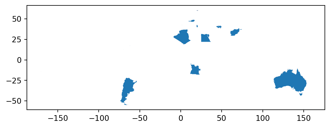

SF objects

Geoseries use the “simple features” standard to describe the shape and location of geographical objects.

A GeoDataFrame can have any number of columns with geographic data but it has a single geometry “active” at a time, which can be set with .set_geometry - the standard is to call it geometry as well

type(world.geometry)

geopandas.geoseries.GeoSeries

type(world["geometry"])

geopandas.geoseries.GeoSeries

Points are defined by two coordinates (x, y) :

point = gpd.GeoSeries.from_wkt(["POINT(0 0)"])

# WKT stands for "well known text" representation, a standard markup language to represent vector geometry object

point

0    POINT (0 0)
dtype: geometry

point.plot()

A line is an array of points

line = gpd.GeoSeries.from_wkt(["LINESTRING(0 0, 10 10, -10 10, 25 20)"])
line.plot()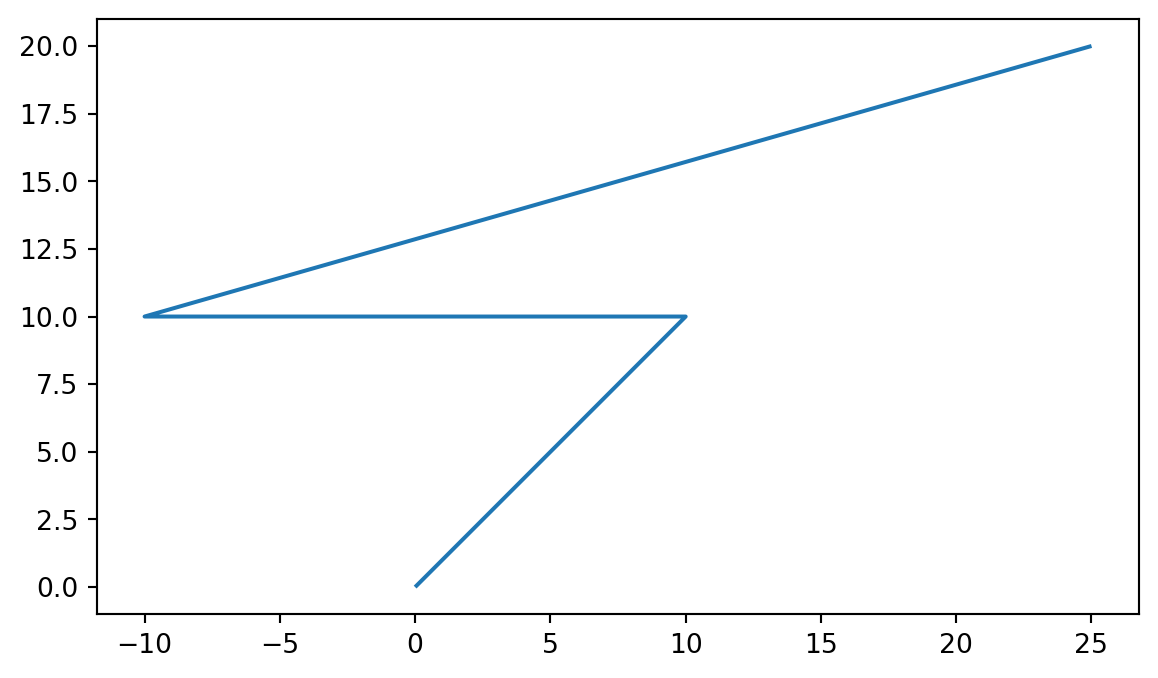

Polygons are areas defined by a line string whose first and last point are the same

polygon = gpd.GeoSeries.from_wkt(["POLYGON((0 0, 10 10, -10 10, -10 3, 0 0))"])
polygon.plot()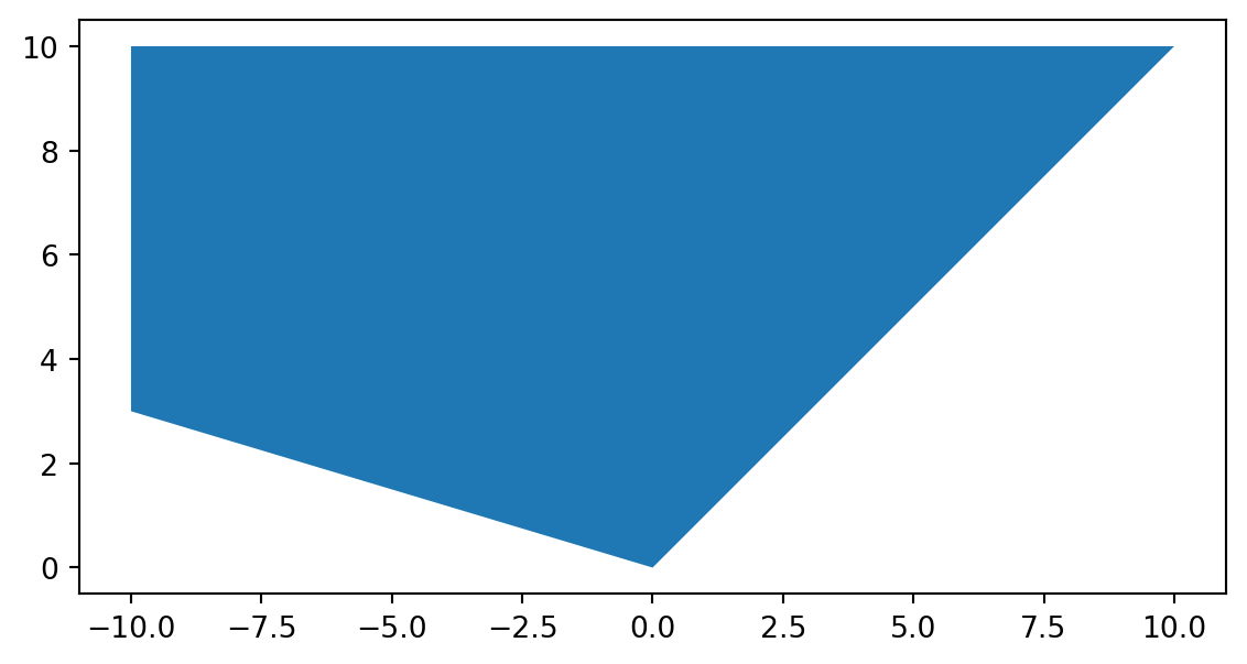  

MultiPoints, MultiLineStrings and MultiPolygons are simply an array of Points, LineStrings or Polygons

france = world[world["NAM_0"] == "France"]
france["geometry"]

70     MULTIPOLYGON (((55.38132 -20.89142, 55.38385 -...
83     MULTIPOLYGON (((45.14231 -12.92269, 45.13968 -...
92     MULTIPOLYGON (((-1.13006 49.2843, -1.13082 49....
200    MULTIPOLYGON (((-61.59331 15.87191, -61.59649 ...
202    MULTIPOLYGON (((-52.24012 4.23658, -52.23805 4...
209    MULTIPOLYGON (((-61.00384 14.57096, -61.00338 ...
Name: geometry, dtype: geometry

france.explore()

Make this Notebook Trusted to load map: File -> Trust Notebook

Type	Use Case	Example
Point	Locations	Cities, sensors
LineString	Routes	Roads, rivers
Polygon	Areas	Countries, buildings
MultiPolygon	Disjoint areas	Archipelagos, split regions

Practise

• Load the country dataset
• Filter to only NON members of the WB (WB_STATUS != “Member State”)
• Plot them

world = gpd.read_file("./data/countries.gpkg")
world_bank_members = world[world['WB_STATUS'] != "Member State"]
world_bank_members.explore()

Make this Notebook Trusted to load map: File -> Trust Notebook

Manipulation

france = world[world["NAM_0"] == "France"].reset_index().to_crs(epsg = 3857)
france_geometry = france.geometry.unary_union

paris_df = pd.DataFrame({
    "ADMIN" : ["Paris"],
    "Latitude" : [48.85548],
    "Longitude" : [2.347421]
    })

paris = gpd.GeoDataFrame(
    paris_df,
    geometry = gpd.points_from_xy(paris_df.Longitude, paris_df.Latitude),
    crs = "EPSG:4326"
    ).to_crs(epsg = 3857)

france.explore()

/tmp/ipykernel_26875/3394447242.py:2: DeprecationWarning: The 'unary_union' attribute is deprecated, use the 'union_all()' method instead.
  france_geometry = france.geometry.unary_union

Make this Notebook Trusted to load map: File -> Trust Notebook

• Buffer : all points within a certain distance of an object

area_around_paris = paris.buffer(distance = 500 * 1000)
base = france.plot(color = "grey")
area_around_paris.plot(ax = base, color = "red")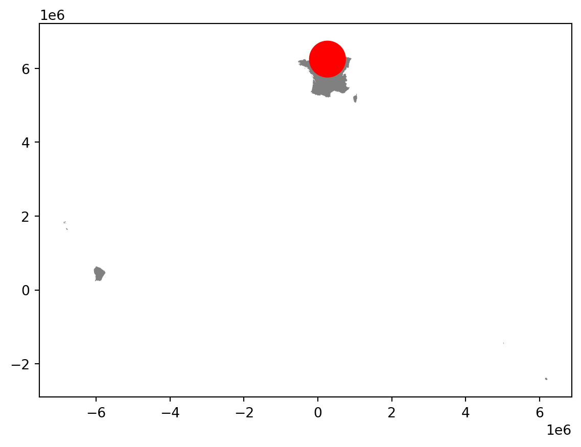

• Intersection of two objects: points within both objects

northern_france = area_around_paris.geometry.intersection(france_geometry)
base = france.plot(color = "grey")
northern_france.plot(ax = base, color = "red")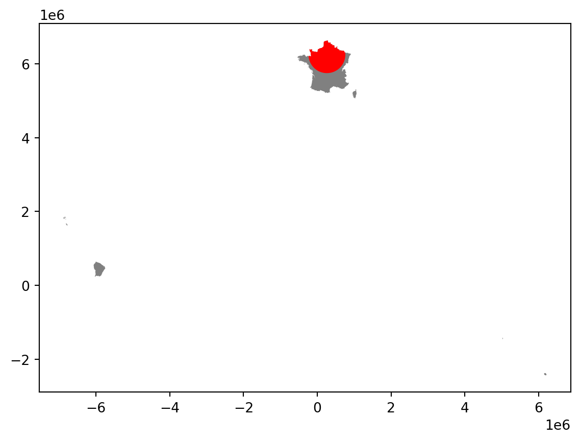

• Simplify : create a simplified geometry

northern_france_simplified = northern_france.simplify(50000)

base = northern_france.plot(color = "grey")
northern_france_simplified.plot(ax = base)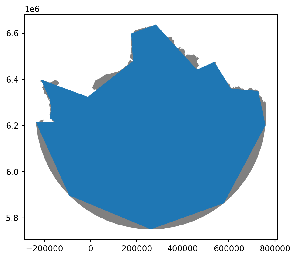

• Difference

france_geometry.difference(northern_france).plot()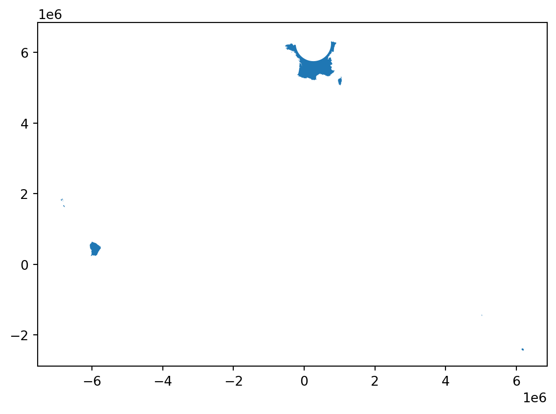

• Centroid, hull, enveloppe

metropolitan_france = paris \
    .buffer(distance = 5000 * 1000) \
    .geometry.intersection(france_geometry)

base = metropolitan_france.plot(color = "grey")
metropolitan_france.centroid.plot(ax = base)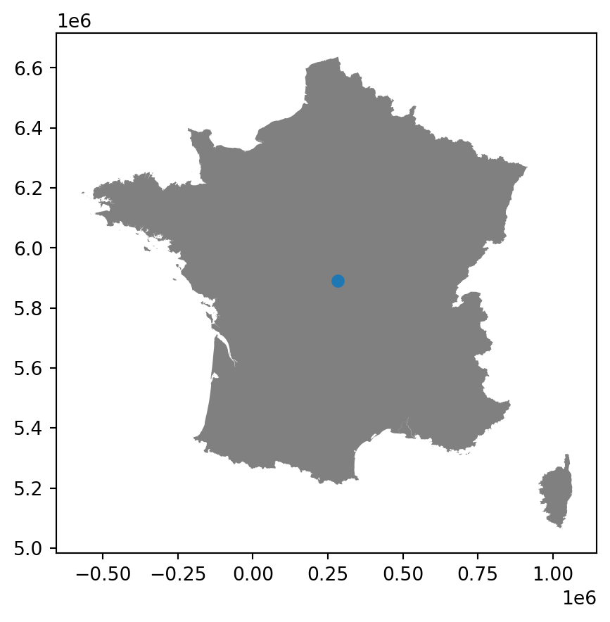

base = metropolitan_france.plot(color = "grey")
metropolitan_france.convex_hull.plot(ax = base, alpha = .5)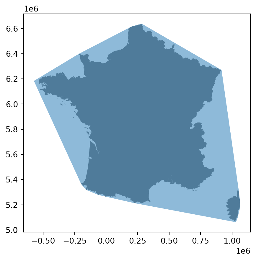

base = metropolitan_france.plot(color = "grey")
metropolitan_france.envelope.plot(ax = base, alpha = .5)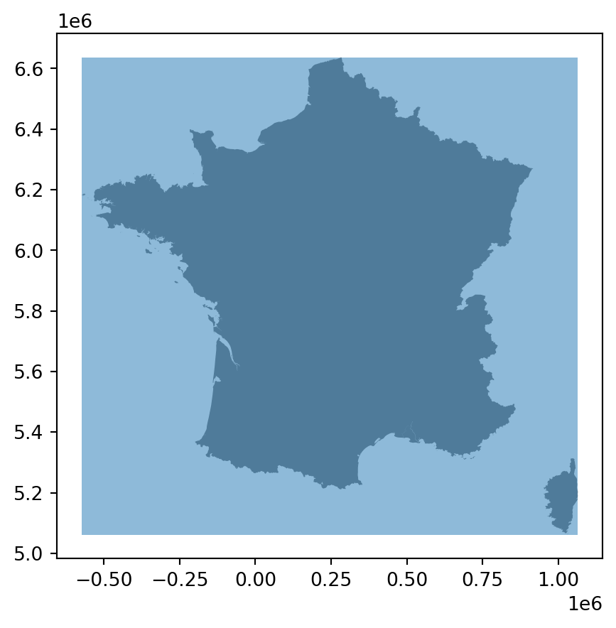

• Dissolve:
  • aggregate attributes
  • join geometries using union_all

population_data = pd.read_csv("https://gist.githubusercontent.com/alex4321/0a2da1d87205a6c29f0d4235e9523565/raw/ce9fa5637a670e846a37d9a3d9bf36aea547314d/world-population.csv").rename(columns = {"CCA3": "ISO_A3", "2022 Population": "latest_population"}) [["ISO_A3", "latest_population", "Continent"]]

merged_world = world \
    .merge(population_data, on = "ISO_A3", how = "left")

merged_world

	ISO_A3	ISO_A2	WB_A3	HASC_0	GAUL_0	WB_REGION	WB_STATUS	SOVEREIGN	NAM_0	geometry	latest_population	Continent
0	CHN	CN	CHN	CN	147295	EAP	Member State	CHN	China	MULTIPOLYGON (((117.58675 38.59517, 117.58909 ...	1.425887e+09	Asia
1	JPN	JP	JPN	JP	126	Other	Member State	JPN	Japan	MULTIPOLYGON (((137.48411 34.67386, 137.46683 ...	1.239517e+08	Asia
2	KOR	KR	KOR	KR	202	EAP	Member State	KOR	Republic of Korea	MULTIPOLYGON (((126.05363 36.19852, 126.05372 ...	5.181581e+07	Asia
3	PRK	KP	PRK	KP	67	Other	Non Member State	PRK	D. P. R. of Korea	MULTIPOLYGON (((126.95508 38.16282, 126.95184 ...	2.606942e+07	Asia
4	RUS	RU	RUS	RU	204	ECA	Member State	RUS	Russian Federation	MULTIPOLYGON (((130.61904 48.88019, 130.60659 ...	1.447133e+08	Europe
...	...	...	...	...	...	...	...	...	...	...	...	...
259	UMI	UM	UMI	UM	129	Other	Territory	USA	U.S. Minor Outlying Islands (U.S.)	MULTIPOLYGON (((-169.51424 16.75948, -169.5177...	NaN	NaN
260	UMI	UM	UMI	UM	190	Other	Territory	USA	U.S. Minor Outlying Islands (U.S.)	MULTIPOLYGON (((-162.05749 5.87833, -162.05696...	NaN	NaN
261	URY	UY	URY	UY	260	LCR	Member State	URY	Uruguay	MULTIPOLYGON (((-56.65825 -30.20105, -56.65254...	3.422794e+06	South America
262	WLF	WF	WLF	WF	266	Other	Territory	FRA	Wallis and Futuna (Fr.)	MULTIPOLYGON (((-176.24899 -13.30266, -176.247...	1.157200e+04	Oceania
263	WSM	WS	WSM	WS	212	EAP	Member State	WSM	Samoa	MULTIPOLYGON (((-172.40519 -13.45112, -172.400...	2.223820e+05	Oceania

264 rows × 12 columns

merged_world.plot("latest_population")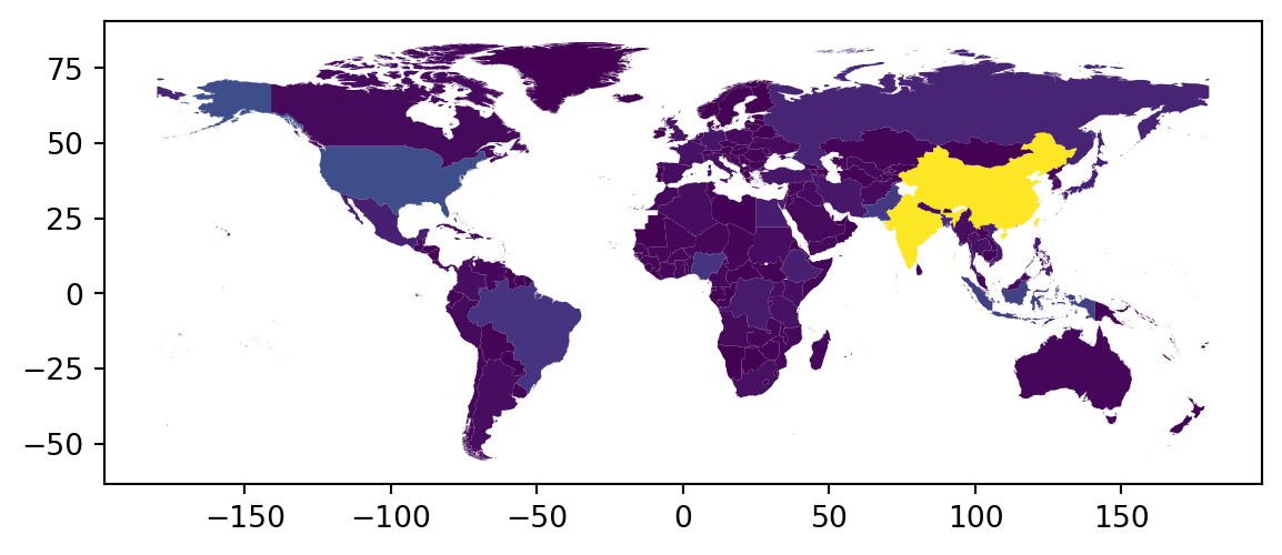

merged_world.plot("Continent")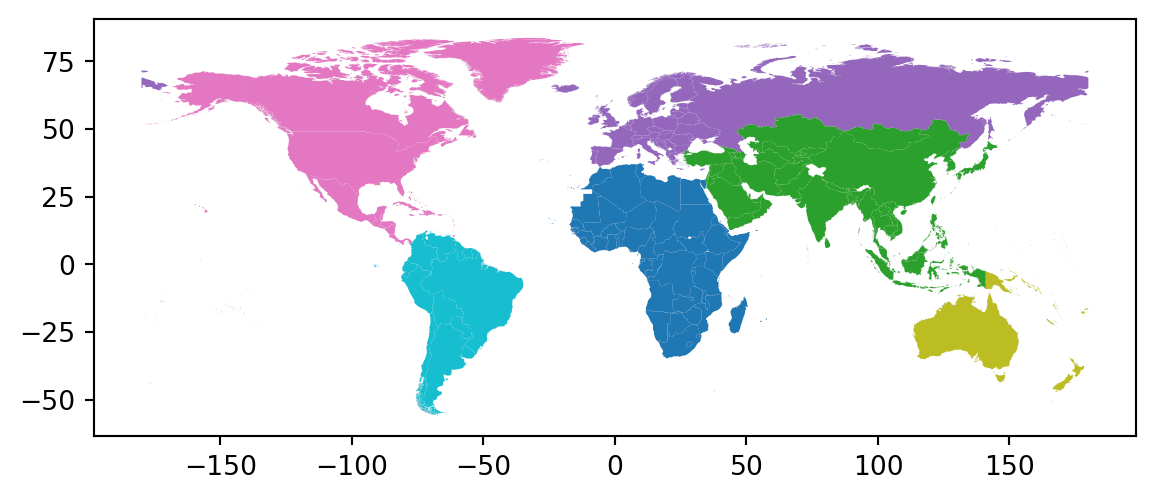

merged_world.groupby("Continent")[['latest_population']].sum().reset_index()

	Continent	latest_population
0	Africa	1.442475e+09
1	Asia	4.697490e+09
2	Europe	1.173320e+09
3	North America	6.002961e+08
4	Oceania	7.121597e+07
5	South America	4.368128e+08

regions = merged_world[["Continent", "latest_population", "geometry"]] \
    .dissolve(by = "Continent", aggfunc = "sum") \
    .reset_index()

regions

	Continent	geometry	latest_population
0	Africa	MULTIPOLYGON (((-16.65703 12.32403, -16.66085 ...	1.442475e+09
1	Asia	MULTIPOLYGON (((43.41959 12.65259, 43.423 12.6...	4.697490e+09
2	Europe	MULTIPOLYGON (((-109.21926 10.28898, -109.2213...	1.173320e+09
3	North America	MULTIPOLYGON (((-157.02337 20.92601, -157.0170...	6.002961e+08
4	Oceania	MULTIPOLYGON (((-176.16808 -44.34635, -176.163...	7.121597e+07
5	South America	MULTIPOLYGON (((-80.83593 -33.75699, -80.83794...	4.368128e+08

regions.plot("latest_population")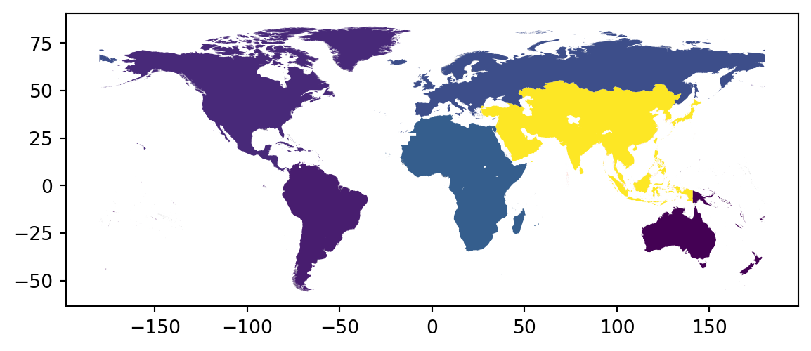

Raster data

Remote sensing tools (eg pictures taken from a satellite) typically output data as a grid of equal-sized cells containing values (eg elevation), where each cell corresponds to a location.

This is known as raster data.

# https://geoservices.ign.fr/bdalti
savoie = rasterio.open('data/savoie.asc', crs = "EPSG:2154")

rasterio.plot.show(savoie)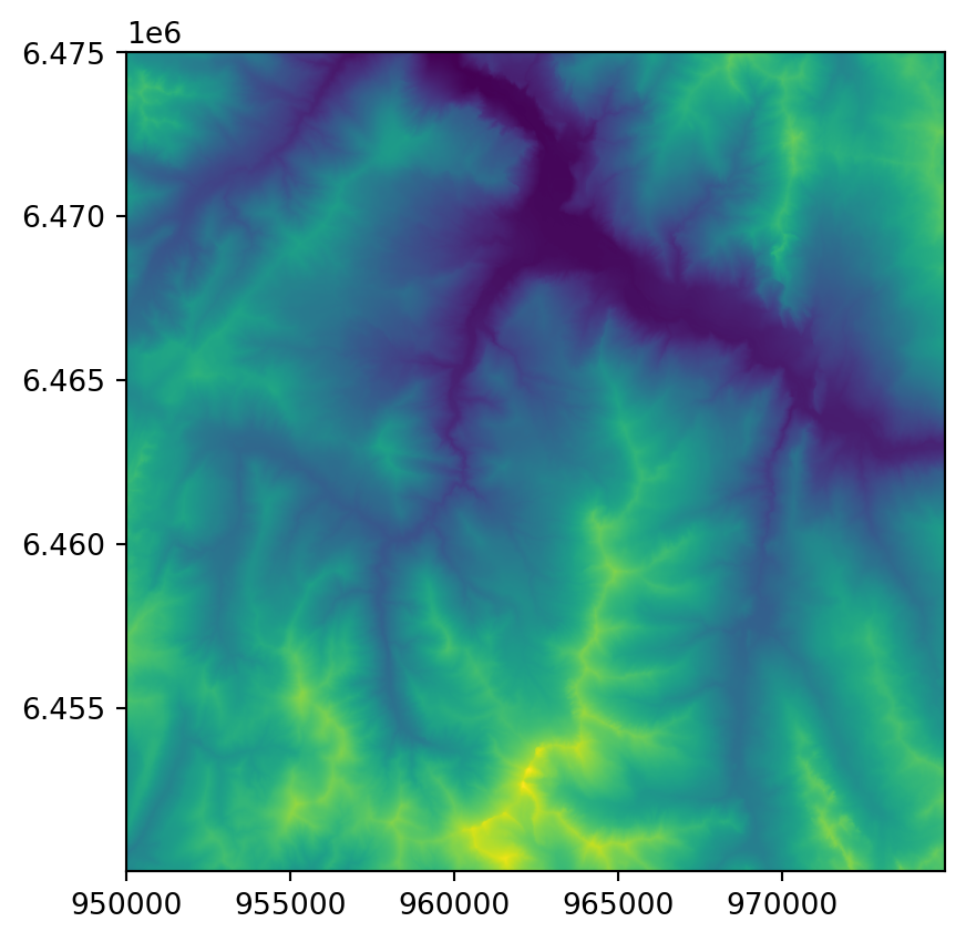

savoie.meta

{'driver': 'AAIGrid',
 'dtype': 'float32',
 'nodata': -99999.0,
 'width': 1000,
 'height': 1000,
 'count': 1,
 'crs': None,
 'transform': Affine(25.0, 0.0, 949987.5,
        0.0, -25.0, 6475012.5)}

fig, ax = plt.subplots(figsize=(12, 10))
rasterio.plot.show(savoie, ax=ax)
metropolitan_france.to_crs(epsg = 2154).boundary.plot(ax = ax)
fig.show()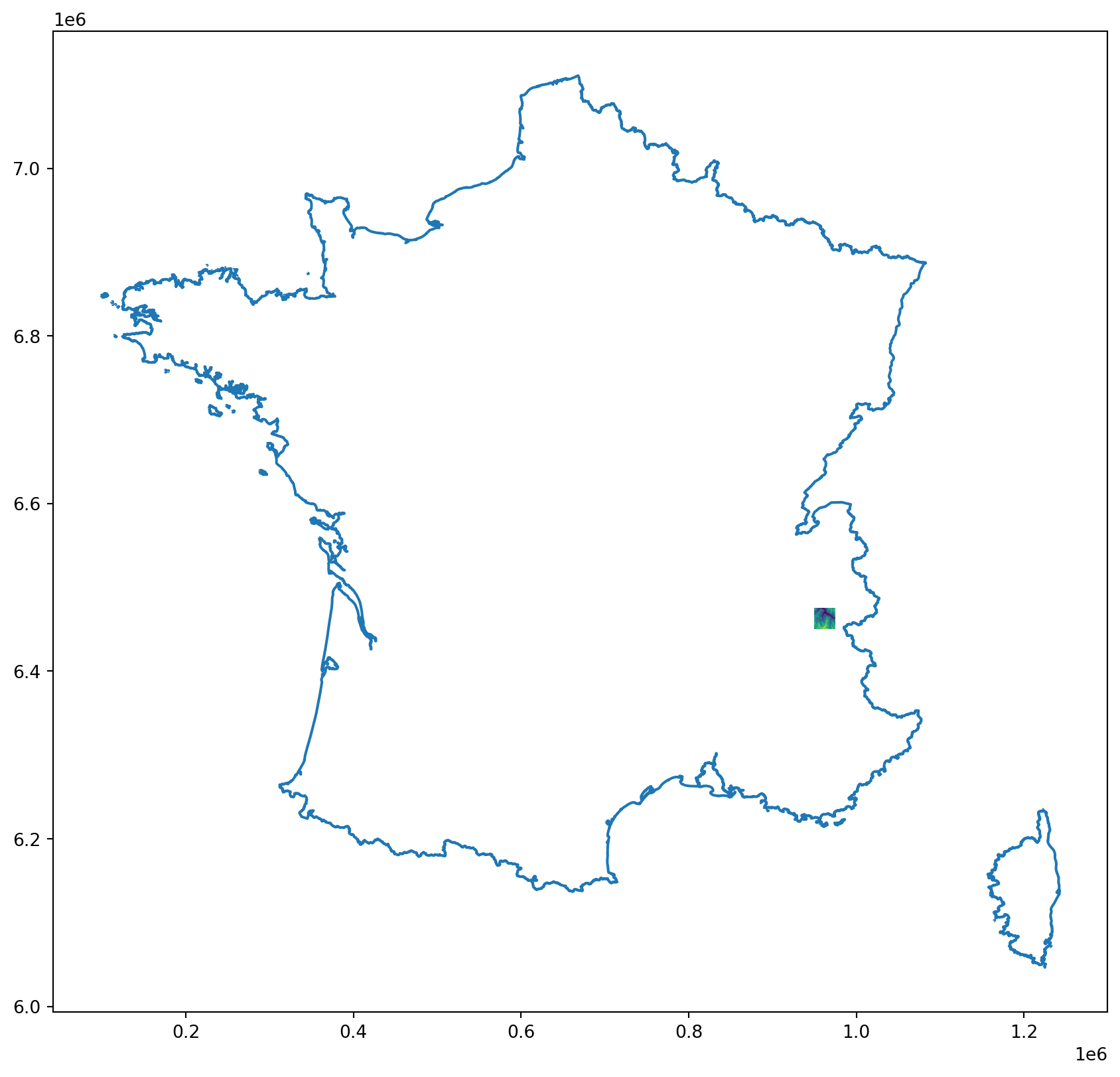

Much like vector data, raster data has: - geometry data: the indices of the cell - attribute data: one or several “bands”

elevation = savoie.read(1)
elevation

array([[2114.4 , 2098.3 , 2085.7 , ..., 2291.3 , 2264.8 , 2245.6 ],
       [2111.  , 2096.4 , 2081.8 , ..., 2297.3 , 2264.5 , 2240.  ],
       [2117.  , 2097.9 , 2082.1 , ..., 2297.7 , 2265.2 , 2237.8 ],
       ...,
       [1876.97, 1882.37, 1888.06, ..., 2647.9 , 2647.7 , 2634.5 ],
       [1870.16, 1874.63, 1879.21, ..., 2643.1 , 2643.2 , 2628.8 ],
       [1864.45, 1868.97, 1871.44, ..., 2642.1 , 2639.  , 2628.7 ]],
      dtype=float32)

This is just a numpy 2D array

np.mean(elevation)

np.float32(1817.3401)

plt.hist(elevation.flatten());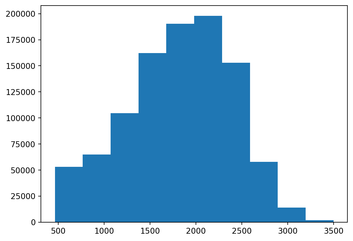

Let’s compute the slope

px, py = np.gradient(elevation, 5)
slope = np.sqrt(px ** 2 + py ** 2) 
slope

array([[3.2909856, 2.8950465, 2.5140684, ..., 5.1322513, 4.570389 ,
        3.999996 ],
       [2.931573 , 2.9202693, 2.654503 , ..., 4.802841 , 5.730144 ,
        4.9616942],
       [4.0383997, 3.6416566, 3.2983723, ..., 6.1214924, 6.0405617,
        5.5834646],
       ...,
       [1.8031999, 1.9270909, 1.7395694, ..., 2.2698996, 1.4103854,
        3.0563245],
       [1.5384195, 1.6169782, 1.7304919, ..., 1.4052721, 1.6738594,
        2.9378042],
       [1.4565113, 1.3304282, 1.5725809, ..., 1.1574012, 1.5815256,
        2.060107 ]], dtype=float32)

rasterio.plot.show(slope, cmap='Reds')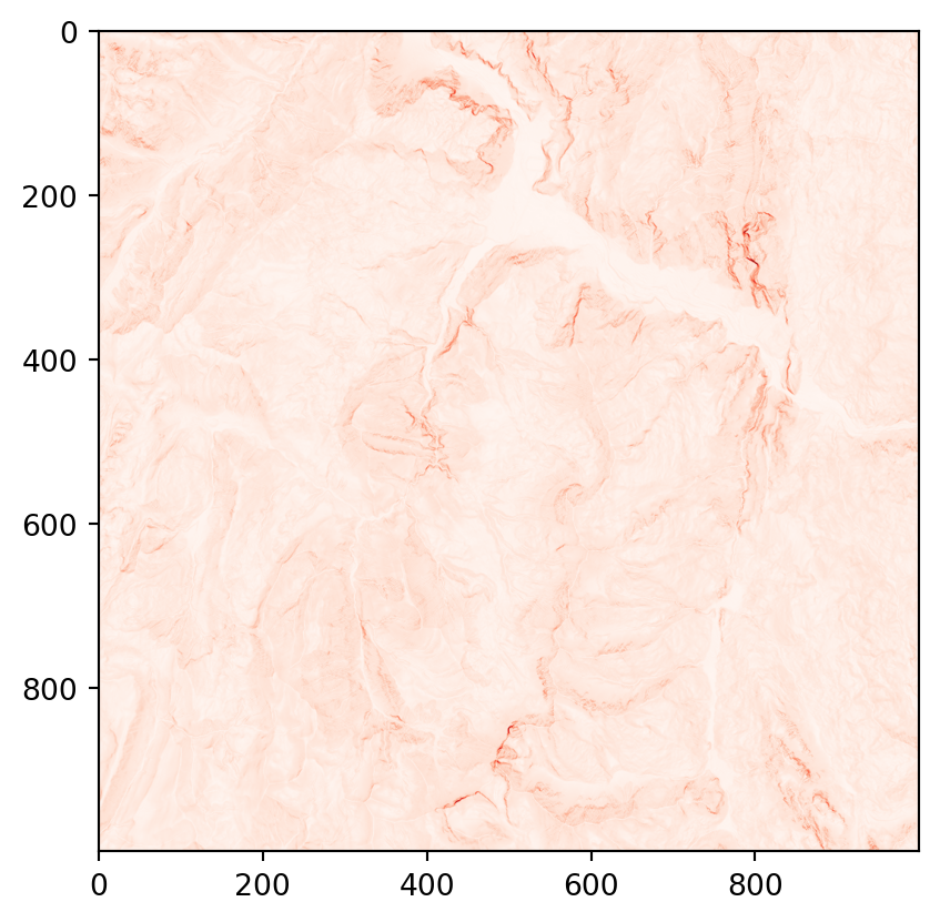

Practice

• Read the raster_savoie.asc file
• Store the first (and only) band (elevation) in a variable
• Create a new numpy.ndarray whose value is 1 when the elevation is above 2000 meters and 0 otherwise
• Plot it

savoie = rasterio.open('data/savoie.asc', crs = "EPSG:2154")
above_2000 = savoie.read(1) > 2000
rasterio.plot.show(above_2000, cmap='Reds')

rasterio.plot.show(above_2000 & (slope > 1e3), cmap='Reds')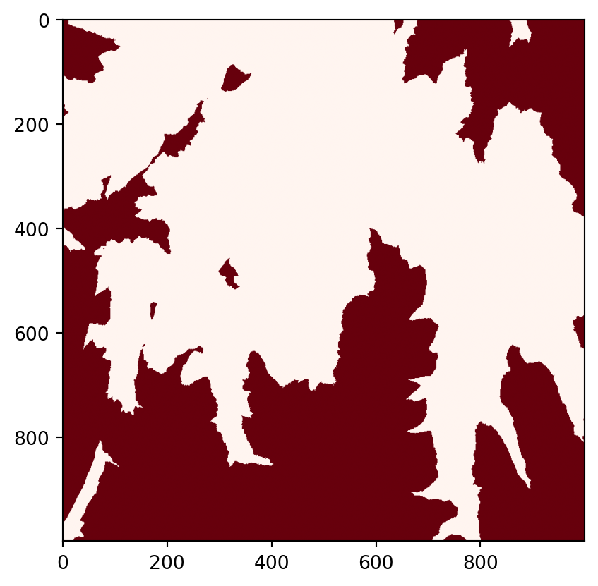

/opt/python/lib/python3.13/site-packages/rasterio/plot.py:375: RuntimeWarning: invalid value encountered in divide
  return (band - imin) / (imax - imin)

CRS

Vector objects have coordinates, for instance (0, 0)

point = gpd.GeoSeries.from_wkt(["POINT(0 0)"])
point

0    POINT (0 0)
dtype: geometry

To go from an actual physical point on Earth surface to coordinates, we need a few things: - a reference shape for the Earth surface, for instance a sphere (but usually an ellipsoid) - axes with a direction & norm to have a 2D or 3D-coordinate system based on the 3D ellipsoid - some way to go from a 3D ellipsoid to a 2D plane with Cartesian coordinates (this is called a projection) - etc.

This is called a coordinate reference system (CRS)

world.geometry.crs

<Geographic 2D CRS: EPSG:4326>
Name: WGS 84
Axis Info [ellipsoidal]:
- Lat[north]: Geodetic latitude (degree)
- Lon[east]: Geodetic longitude (degree)
Area of Use:
- name: World.
- bounds: (-180.0, -90.0, 180.0, 90.0)
Datum: World Geodetic System 1984 ensemble
- Ellipsoid: WGS 84
- Prime Meridian: Greenwich

Here for instance we use the WGS84 ellipsoid and the Pseudo-Mercator projection

Different CRSs have different uses, e.g. Mercator projection is useful for navigation (preserves some from of angles) but distorts size of landmasses.

canada = world[world["NAM_0"] == "Canada"]

ax = canada.plot()
ax.set_title("WGS84, Pseudo Mercator")

Text(0.5, 1.0, 'WGS84, Pseudo Mercator')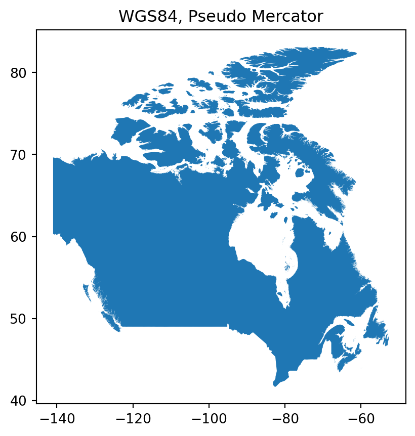

canada_alternative = canada.to_crs(epsg = 6053)
ax = canada_alternative.plot()
ax.set_title(" GR96 / EPSG Arctic zone 3-29 ")

Text(0.5, 1.0, ' GR96 / EPSG Arctic zone 3-29 ')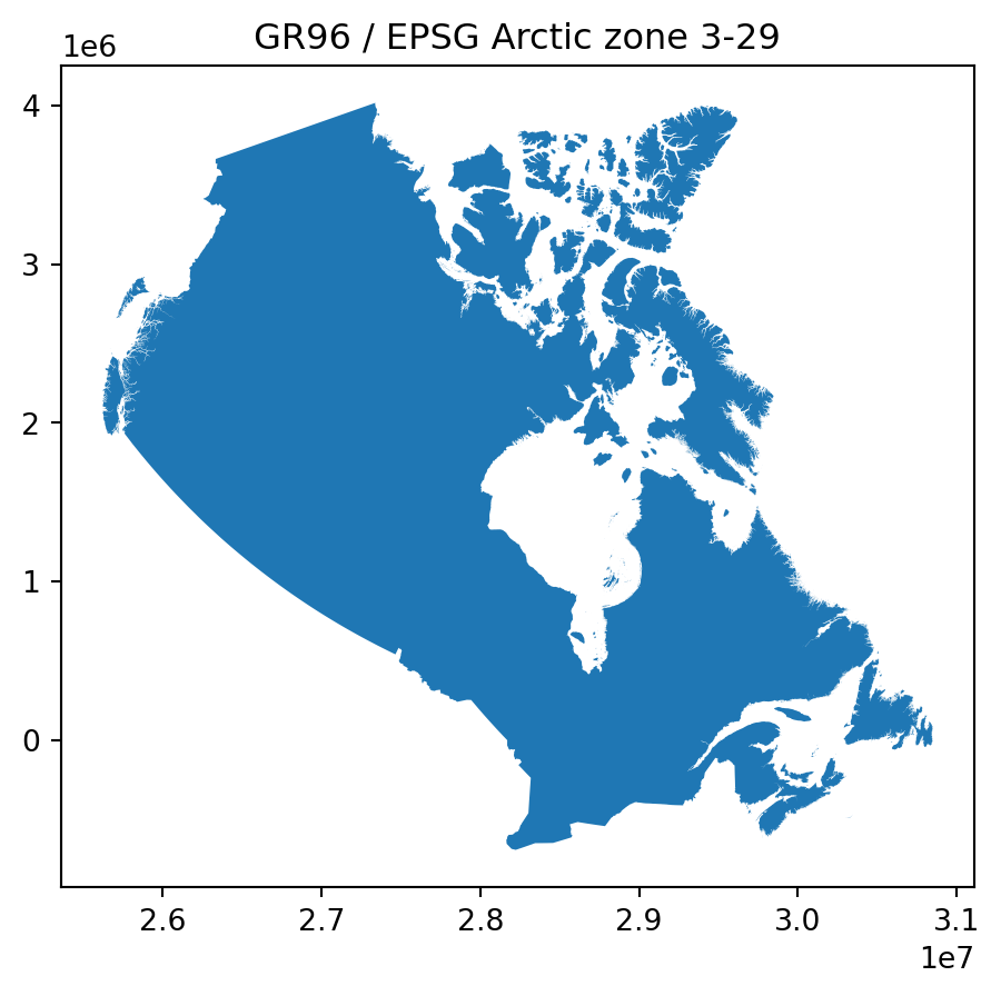

Use the appropriate CRS for your purpose.

If using information from several datasets, make sure to reproject them to the same CRS.

CRS defines how coordinates map to locations on Earth.

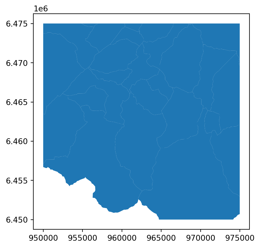
Vector / Raster interactions

from shapely.geometry import mapping
from rasterio.mask import mask

communes_url = "https://raw.githubusercontent.com/makinacorpus/tutorials/refs/heads/master/geospatial-analysis/notebooks/data/communes-73-savoie.geojson"

communes = gpd.read_file(communes_url)  
communes = communes.to_crs(epsg = 2154)

fig, ax = plt.subplots(figsize=(12, 10))
rasterio.plot.show(savoie, ax=ax)
communes.to_crs(epsg = 2154).boundary.plot(ax = ax)
fig.show()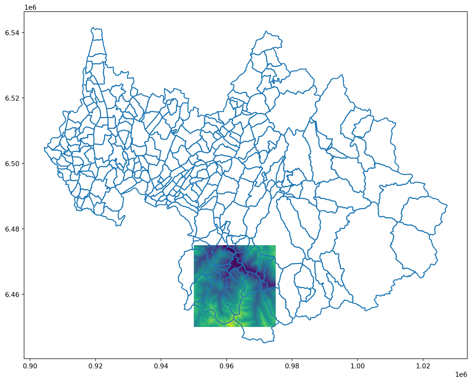

from rasterio.features import rasterize
from shapely.geometry import box, mapping

raster_geom = box(*savoie.bounds)
intersection = communes.union_all().intersection(raster_geom)

out_image, out_transform = mask(savoie, [mapping(intersection)], crop=True)
elevation = out_image[0].astype(float)

communes_clipped = gpd.clip(communes, gpd.GeoSeries([intersection], crs="EPSG:2154"))

rasterio.plot.show(elevation)
communes_clipped.plot()

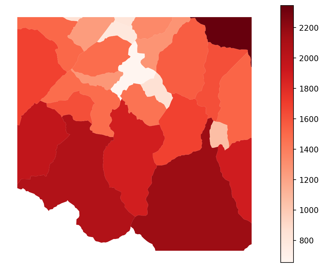
def mean_from_rasterized(geom, arr, transform):
    mask_arr = rasterize([ (mapping(geom), 1) ],
                         out_shape=arr.shape,
                         transform=transform,
                         fill=0,
                         dtype='uint8')
    vals = arr[mask_arr.astype(bool)]
    return float(np.nanmean(vals)) if vals.size else np.nan

communes_clipped["mean_elev_m"] = communes_clipped.geometry.apply(
    lambda g: mean_from_rasterized(g, elevation, out_transform)
)

# 5) Plot choropleth
ax = communes_clipped.plot(column="mean_elev_m", cmap="Reds", legend=True, figsize=(8,6))
ax.set_axis_off()
plt.show()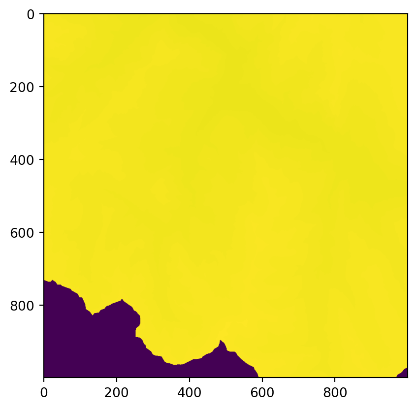

Example recap

• Estimate population at risk from Installations classées pour la protection de l’environnement from census (RP)

pd.read_csv('./data/carreaux_1km_met.csv', sep = ";")

	id_carreau_1km	carreau_traite_secret	depcom_liste	pop	pop0014	pop1564	pop65p	popf	popfr	poph	pophorsue	popmigr0	popmigrfr	popmigrhorsfr	popue
0	FR_CRS3035RES1000mN2031000E4252000	0	2A041	49.366356	7.003686	36.279018	6.083652	23.215187	43.317963	26.151169	4.043924	44.332018	5.034338	0.000000	2.004469
1	FR_CRS3035RES1000mN2032000E4250000	0	2A041	676.462260	85.103524	430.266102	161.092635	339.373519	479.397059	337.088741	134.139430	624.157469	39.345787	4.987735	62.925771
2	FR_CRS3035RES1000mN2032000E4251000	0	2A041	387.944534	82.789564	233.069807	72.085163	194.168349	320.215254	193.776185	48.708632	378.982039	7.971944	0.000000	19.020648
3	FR_CRS3035RES1000mN2032000E4252000	0	2A041	284.853500	52.595460	175.370871	56.887168	147.461899	234.717308	137.391601	24.124283	262.793132	20.079133	0.000000	26.011909
4	FR_CRS3035RES1000mN2033000E4250000	0	2A041	252.713326	25.710928	125.263185	101.739212	143.438133	214.601853	109.275193	22.018474	243.696966	8.025809	0.000000	16.092999
...	...	...	...	...	...	...	...	...	...	...	...	...	...	...	...
374617	FR_CRS3035RES1000mN3132000E3798000	1	59107,59260	13.092919	1.885822	8.811912	2.395185	6.498882	12.256362	6.594038	0.109271	11.360287	1.561412	0.060365	0.727285
374618	FR_CRS3035RES1000mN3132000E3799000	1	59107,59260	6.586305	0.948650	4.432773	1.204882	3.269219	6.165481	3.317086	0.054968	5.714716	0.785458	0.030366	0.365856
374619	FR_CRS3035RES1000mN3132000E3800000	1	59260	1.884937	0.167971	1.182151	0.534816	1.090212	1.800749	0.794725	0.039001	1.763911	0.078003	0.000000	0.045186
374620	FR_CRS3035RES1000mN3134000E3796000	1	59107	11.843281	1.705832	7.970869	2.166579	5.878603	11.086568	5.964677	0.098842	10.276017	1.412384	0.054604	0.657871
374621	FR_CRS3035RES1000mN3134000E3799000	1	59107	2.009338	0.289412	1.352342	0.367583	0.997367	1.880954	1.011971	0.016770	1.743435	0.239626	0.009264	0.111615

374622 rows × 15 columns

rp = pd.read_csv('./data/carreaux_1km_met.csv', sep = ";")

s = rp['id_carreau_1km'].astype(str).str.replace(' ', '').str.upper()
s2 = (
    s
    .str.replace('FR_CRS', '', regex=False)   
    .str.replace('RES', '|', regex=False)     
    .str.replace('M', '', regex=False)        
    .str.replace('N', '|', regex=False)       
    .str.replace('E', '|', regex=False)       
)

parts = s2.str.split('|')
rp['epsg'] = pd.to_numeric(parts.str[0], errors='coerce').astype('Int64')
rp['res_m'] = pd.to_numeric(parts.str[1], errors='coerce')
rp['y'] = pd.to_numeric(parts.str[2], errors='coerce')
rp['x'] = pd.to_numeric(parts.str[3], errors='coerce')

res = rp['res_m']

xmin = rp['x']
ymin = rp['y']
xmax = xmin + res
ymax = ymin + res

from shapely.geometry import box

geoms = [box(xmin.loc[idx], ymin.loc[idx], xmax.loc[idx], ymax.loc[idx]) for idx in rp.index]
rp['geometry'] = geoms

epsg_code = int(rp['epsg'].dropna().unique()[0])  
gdf = gpd.GeoDataFrame(rp, geometry='geometry', crs=f'EPSG:{epsg_code}')
gdf = gdf[["pop", "geometry"]]

GRID = 5000.0

bounds = gdf.geometry.bounds
gdf = gdf.assign(
    minx=bounds['minx'],
    miny=bounds['miny']
)

gdf['x25_origin'] = (np.floor(gdf['minx'] / GRID) * GRID).astype(int)
gdf['y25_origin'] = (np.floor(gdf['miny'] / GRID) * GRID).astype(int)

gdf['cell_id_25km'] = gdf['x25_origin'].astype(str) + '_' + gdf['y25_origin'].astype(str)

gdf25 = gdf.dissolve(
    by='cell_id_25km',
    aggfunc={'pop': 'sum', 'x25_origin': 'first', 'y25_origin': 'first'}
).reset_index()

from shapely.geometry import box
gdf25['geometry'] = gdf25.apply(
    lambda r: box(r['x25_origin'], r['y25_origin'],
                  r['x25_origin'] + GRID, r['y25_origin'] + GRID),
    axis=1
)

# keep / reorder columns as desired
gdf = gdf25[['cell_id_25km', 'pop', 'geometry']]

icpe = pd.read_csv("./data/icpe.csv", sep = ";")
seveso = icpe[icpe["lib_seveso"] == 'Seveso seuil haut']

seveso[['x', 'y']] = seveso[['x', 'y']].apply(pd.to_numeric, errors='coerce')

epsgs = seveso['code_epsg'].dropna().unique()
epsg = int(epsgs[0])

seveso = gpd.GeoDataFrame(
    seveso,
    geometry=gpd.points_from_xy(seveso['x'], seveso['y']),
    crs=f"EPSG:{epsg}"
    )

seveso = seveso[["code_aiot", "geometry"]]

/tmp/ipykernel_26875/758005914.py:1: DtypeWarning: Columns (5,7) have mixed types. Specify dtype option on import or set low_memory=False.
  icpe = pd.read_csv("./data/icpe.csv", sep = ";")
/tmp/ipykernel_26875/758005914.py:4: SettingWithCopyWarning: 
A value is trying to be set on a copy of a slice from a DataFrame.
Try using .loc[row_indexer,col_indexer] = value instead

See the caveats in the documentation: https://pandas.pydata.org/pandas-docs/stable/user_guide/indexing.html#returning-a-view-versus-a-copy
  seveso[['x', 'y']] = seveso[['x', 'y']].apply(pd.to_numeric, errors='coerce')

metric_crs = gdf.estimate_utm_crs()
gdf = gdf.to_crs(metric_crs)
seveso = seveso.to_crs(metric_crs)

seveso_buff = seveso.copy()
seveso_buff['geometry'] = seveso_buff.geometry.buffer(10000) 

seveso_buff_viz = seveso_buff.to_crs(4326).copy()
seveso_buff_viz.geometry = seveso_buff_viz.geometry.simplify(0.001, preserve_topology=True)
seveso_buff_viz[["code_aiot", "geometry"]].explore()

Make this Notebook Trusted to load map: File -> Trust Notebook

union = seveso.geometry.buffer(10000).union_all()   
gdf['within_1km'] = gdf.geometry.intersects(union)
gdf_near = gdf[gdf['within_1km']]

gdf_near.head()

	cell_id_25km	pop	geometry	within_1km
37	3245000_2905000	657.700570	POLYGON ((-58807.844 5377655.605, -59280.534 5...	True
38	3245000_2910000	12957.515668	POLYGON ((-59280.534 5382633.946, -59753.374 5...	True
39	3245000_2915000	3880.915251	POLYGON ((-59753.374 5387612.263, -60226.366 5...	True
53	3250000_2900000	1600.406535	POLYGON ((-53326.211 5373171.381, -53798.657 5...	True
54	3250000_2905000	65.936681	POLYGON ((-53798.657 5378149.58, -54271.256 53...	True

gdf_near_viz = gdf_near.to_crs(4326).copy()
gdf_near_viz.geometry = gdf_near_viz.geometry.simplify(0.0005, preserve_topology=True)
gdf_near_viz[["pop", "geometry"]].sample(min(3000, len(gdf_near_viz))).explore(column='pop')

Make this Notebook Trusted to load map: File -> Trust Notebook

#import cartogram

#c = cartogram.Cartogram(gdf_near, "pop")

#c.explore()

Recap exercise

• Small exercise inspired by Le Monde’s analysis of pesticide exposure near French schools:
  • https://www.lemonde.fr/les-decodeurs/article/2025/12/18/votre-ecole-est-elle-soumise-a-une-forte-pression-pesticide-explorez-notre-carte_6658475_4355771.html
  • https://assets-decodeurs.lemonde.fr/decodeurs/assets/20251102_ecoles_pesticides/Barometre_Ecoles_Pesticides_Methodologie.pdf
• Schools in Bretagne exposed to contaminated water

Load school data

• TODO: load “./data/fr-en-annuaire-education.csv”, keep only schools in Bretagne, set the geometry, plot them

schools = (
    pd.read_csv("./data/fr-en-annuaire-education.csv", sep=';') \
    .query("Libelle_region == 'Bretagne'") \
    .query("Type_etablissement == 'Ecole'")
    )

crs = "EPSG:2154"

schools =  gpd.GeoDataFrame(
    schools,
    geometry = gpd.points_from_xy(schools["coordX_origine"], schools["coordY_origine"]),
    crs = crs
    )

schools = schools[["Nom_etablissement", "Code_commune", "geometry"]]

schools

/tmp/ipykernel_26875/2375027476.py:2: DtypeWarning: Columns (59,62) have mixed types. Specify dtype option on import or set low_memory=False.
  pd.read_csv("./data/fr-en-annuaire-education.csv", sep=';') \

	Nom_etablissement	Code_commune	geometry
925	Ecole primaire publique de Plaine Haute	22170	POINT (267313.7 6831928.6)
926	Ecole primaire publique Montafilan	22180	POINT (314176.9 6828071.4)
927	Ecole élémentaire publique Vent d'Eveil	22185	POINT (300008.9 6821134.8)
928	Ecole primaire publique J. Le Morvan	22198	POINT (221321.9 6872158)
929	Ecole élémentaire publique Louis Guilloux	22215	POINT (272319.5 6836442.5)
...	...	...	...
64870	Ecole élémentaire publique Jean Moulin	29235	POINT (153471.3 6837764.6)
64871	Ecole primaire publique Renée Le Née	29080	POINT (164166.2 6827533.7)
64872	Ecole primaire publique Ferdinand Buisson	29103	POINT (164323.2 6841605.7)
64873	Ecole primaire publique de Locmélar	29131	POINT (178406.2 6840296.8)
64874	Ecole maternelle publique Le Quinquis	29232	POINT (173342.3 6788298.9)

2289 rows × 3 columns

Load water quality data

• TODO: read oeb_pesticides_eau_surface_caracterisation_site_bretagne.csv, keep lines whose annee == 2024, concentration_max

water_quality = (
    pd.read_csv("./data/oeb_pesticides_eau_surface_caracterisation_site_bretagne.csv", sep = ";") \
    .query("serie == 'concentration_max'")
    .query("annee == 2024")
)

water_quality = water_quality[["resultat", "code_commune"]]

water_quality

/tmp/ipykernel_26875/4116893605.py:2: DtypeWarning: Columns (14) have mixed types. Specify dtype option on import or set low_memory=False.
  pd.read_csv("./data/oeb_pesticides_eau_surface_caracterisation_site_bretagne.csv", sep = ";") \

	resultat	code_commune
317	0.970	22218
452	0.998	35110
557	1.200	35176
812	0.550	22283
2147	0.670	44067
...	...	...
138557	1.865	22076
139472	0.920	29170
140132	0.960	35223
140567	0.424	35150
140732	1.280	35265

324 rows × 2 columns

Load commune geometry

• TODO: read adminexpress-cog-simpl-000-2025.gpkg with the argument layer == “commune”; filter insee_reg == “53” (Bretagne) ; keep insee_com & geometry

communes = (
    gpd.read_file("./data/adminexpress-cog-simpl-000-2025.gpkg", layer = "commune")
    .query("insee_reg == '53'")
    )

communes = communes[["insee_com", "geometry"]]

communes

	insee_com	geometry
12	29239	POLYGON ((-4.0071 48.724, -4.01127 48.71663, -...
22	29003	POLYGON ((-4.52821 48.03732, -4.53447 48.04191...
34	22332	POLYGON ((-2.52008 48.402, -2.5204 48.40597, -...
51	22241	POLYGON ((-2.6525 48.11972, -2.65719 48.11523,...
142	22228	POLYGON ((-3.40517 48.56702, -3.41036 48.56943...
...	...	...
34618	35076	POLYGON ((-1.79405 48.08095, -1.79678 48.07984...
34633	56007	POLYGON ((-3.01282 47.6667, -3.01677 47.66398,...
34646	35193	POLYGON ((-1.74708 48.24053, -1.74013 48.23765...
34737	29023	POLYGON ((-3.89542 48.63856, -3.88662 48.63543...
34741	56186	POLYGON ((-3.11963 47.503, -3.12627 47.5044, -...

1202 rows × 2 columns

Merge water_quality & communes as a single geo dataframe

water_quality['code_commune'] = water_quality['code_commune'].astype(str)
communes['insee_com'] = communes['insee_com'].astype(str)

merged = water_quality.merge(
    communes[['insee_com', 'geometry']],
    left_on='code_commune',
    right_on='insee_com',
    how='left'
)

merged_gdf = gpd.GeoDataFrame(merged, geometry='geometry', crs=getattr(communes, 'crs', None))

merged_gdf = merged_gdf.drop(columns=['insee_com'])

merged_gdf

	resultat	code_commune	geometry
0	0.970	22218	POLYGON ((-3.26954 48.83397, -3.27504 48.8215,...
1	0.998	35110	POLYGON ((-1.62246 48.30324, -1.60766 48.30622...
2	1.200	35176	POLYGON ((-1.89211 47.85603, -1.89291 47.84882...
3	0.550	22283	POLYGON ((-3.1567 48.65757, -3.15227 48.65345,...
4	0.670	44067	None
...	...	...	...
319	1.865	22076	POLYGON ((-2.40028 48.53481, -2.39625 48.53525...
320	0.920	29170	POLYGON ((-4.18875 47.9296, -4.17598 47.91978,...
321	0.960	35223	POLYGON ((-2.1227 47.96356, -2.11914 47.9608, ...
322	0.424	35150	POLYGON ((-1.2223 48.33203, -1.21855 48.3303, ...
323	1.280	35265	POLYGON ((-1.88293 48.38158, -1.88999 48.37141...

324 rows × 3 columns

Create a single geometry with all communes whose resultat >= 1

• TODO: filter the merge gdf to keep only lines with resultat >= 1, then create a single geometry from each remaining line

poor_water_quality_zone = (
    merged_gdf \
    .query("resultat >= 1")
    )

poor_water_quality_zone = poor_water_quality_zone[~poor_water_quality_zone["geometry"].isna()]

poor_water_quality_zone = poor_water_quality_zone.dissolve().reset_index(drop=True)

poor_water_quality_zone.explore()

Make this Notebook Trusted to load map: File -> Trust Notebook

Compute which schools are less than 20km from the poor_water_quality_zone

• TODO:
  • put the two in the same CRS
  • get a single geometry using poor_water_quality_zone.geometry.unary_union
  • compute the distance from schools to poor_water_quality_zone using schools.geometry.distance(poor_water_quality_zone)

threshold = 10 * 1e3

utm = schools.estimate_utm_crs()
schools = schools.to_crs(utm)
poor_water_quality_zone = poor_water_quality_zone.to_crs(utm)
poor_water_quality_zone = poor_water_quality_zone.geometry.unary_union

schools = schools[schools.geometry.is_valid].copy()

schools['distance_m'] = schools.geometry.distance(poor_water_quality_zone)
schools['near_mp'] = schools['distance_m'] <= threshold

schools.explore(
    column='near_mp',
    categorical=True,
    cmap=['red', 'blue'],
    legend=True,
    marker_kwds={'radius': 4, 'fill_opacity': 0.9}
)

/tmp/ipykernel_26875/788482969.py:6: DeprecationWarning: The 'unary_union' attribute is deprecated, use the 'union_all()' method instead.
  poor_water_quality_zone = poor_water_quality_zone.geometry.unary_union

Make this Notebook Trusted to load map: File -> Trust Notebook