Spatial Statistics

Spatial statistics

Outline for this part: - Graphs & spatial weight matrices - Spatial autocorrelation - Standard geographic regression models

import numpy as np
from pysal.lib import weights
import pandas as pd
import shapely as sp
import contextily as ctx
import geopandas as gpd
import networkx as nx
import matplotlib.pyplot as plt
import esda
from splot.esda import plot_moran, lisa_cluster
from pysal.model import spreg

constituencies_shapes = gpd.read_file("./data/constituencies_shape/circonscriptions_legislatives_030522.shp")
constituencies_shapes = constituencies_shapes[~constituencies_shapes["id_circo"].str.startswith("97")]
constituencies_shapes.explore()

Make this Notebook Trusted to load map: File -> Trust Notebook

constituencies_x = pd.read_csv("./data/constituencies_x.csv")
constituencies_x["id_circo"] = constituencies_x["id_circo"].astype(str).str[0:2] + constituencies_x["id_circo"].astype(str).str[3:5]
constituencies_y = pd.read_csv("./data/constituencies_y.csv")

constituencies = constituencies_shapes \
    .merge(constituencies_x, on = "id_circo", how = "left") \
    .merge(constituencies_y, on = "id_circo", how = "left")         

constituencies

	id_circo	dep	libelle	geometry	Nom de la circonscription	mean_age	unemployement_rate	D1_diff	D9_diff	rpt_D9_D1_diff	vote_share_rn
0	3803	38	Isère - 3e circonscription	MULTIPOLYGON (((5.70136 45.18796, 5.70136 45.1...	Isère - 3e circonscription	38.1	7.2	10530	36370	3.5	20.41
1	3801	38	Isère - 1re circonscription	MULTIPOLYGON (((5.74302 45.16638, 5.74259 45.1...	Isère - 1re circonscription	39.8	5.4	12080	51150	4.2	14.39
2	3810	38	Isère - 10e circonscription	MULTIPOLYGON (((5.67138 45.47904, 5.66725 45.4...	Isère - 10e circonscription	37.8	6.1	12240	36130	3	38.43
3	3804	38	Isère - 4e circonscription	MULTIPOLYGON (((5.80147 44.70678, 5.77463 44.6...	Isère - 4e circonscription	41.9	4.5	13160	39110	3	28.41
4	3802	38	Isère - 2e circonscription	MULTIPOLYGON (((5.87334 45.09739, 5.88031 45.0...	Isère - 2e circonscription	39.0	5.8	11760	37610	3.2	27.67
...	...	...	...	...	...	...	...	...	...	...	...
534	0502	05	Hautes-Alpes - 2e circonscription	MULTIPOLYGON (((6.23277 44.46288, 6.24026 44.4...	Hautes-Alpes - 2e circonscription	44.6	3.8	11980	35190	2.9	29.44
535	0401	04	Alpes-de-Haute-Provence - 1re circonscription	MULTIPOLYGON (((6.84988 43.9141, 6.83595 43.91...	Alpes de Haute-Provence - 1re circonscription	45.9	6.0	11310	34120	3	38.50
536	4204	42	Loire - 4e circonscription	MULTIPOLYGON (((4.54255 45.24218, 4.53626 45.2...	Loire - 4e circonscription	41.9	4.9	12140	34470	2.8	38.62
537	0703	07	Ardèche - 3e circonscription	POLYGON ((4.05709 44.36415, 4.05709 44.36415, ...	Ardèche - 3e circonscription	46.7	7.3	10880	33580	3.1	32.02
538	0501	05	Hautes-Alpes - 1re circonscription	MULTIPOLYGON (((6.26146 44.5461, 6.26146 44.54...	Hautes-Alpes - 1re circonscription	44.5	5.4	11770	35350	3	32.56

539 rows × 11 columns

constituencies.set_index('id_circo')

	dep	libelle	geometry	Nom de la circonscription	mean_age	unemployement_rate	D1_diff	D9_diff	rpt_D9_D1_diff	vote_share_rn
id_circo
3803	38	Isère - 3e circonscription	MULTIPOLYGON (((5.70136 45.18796, 5.70136 45.1...	Isère - 3e circonscription	38.1	7.2	10530	36370	3.5	20.41
3801	38	Isère - 1re circonscription	MULTIPOLYGON (((5.74302 45.16638, 5.74259 45.1...	Isère - 1re circonscription	39.8	5.4	12080	51150	4.2	14.39
3810	38	Isère - 10e circonscription	MULTIPOLYGON (((5.67138 45.47904, 5.66725 45.4...	Isère - 10e circonscription	37.8	6.1	12240	36130	3	38.43
3804	38	Isère - 4e circonscription	MULTIPOLYGON (((5.80147 44.70678, 5.77463 44.6...	Isère - 4e circonscription	41.9	4.5	13160	39110	3	28.41
3802	38	Isère - 2e circonscription	MULTIPOLYGON (((5.87334 45.09739, 5.88031 45.0...	Isère - 2e circonscription	39.0	5.8	11760	37610	3.2	27.67
...	...	...	...	...	...	...	...	...	...	...
0502	05	Hautes-Alpes - 2e circonscription	MULTIPOLYGON (((6.23277 44.46288, 6.24026 44.4...	Hautes-Alpes - 2e circonscription	44.6	3.8	11980	35190	2.9	29.44
0401	04	Alpes-de-Haute-Provence - 1re circonscription	MULTIPOLYGON (((6.84988 43.9141, 6.83595 43.91...	Alpes de Haute-Provence - 1re circonscription	45.9	6.0	11310	34120	3	38.50
4204	42	Loire - 4e circonscription	MULTIPOLYGON (((4.54255 45.24218, 4.53626 45.2...	Loire - 4e circonscription	41.9	4.9	12140	34470	2.8	38.62
0703	07	Ardèche - 3e circonscription	POLYGON ((4.05709 44.36415, 4.05709 44.36415, ...	Ardèche - 3e circonscription	46.7	7.3	10880	33580	3.1	32.02
0501	05	Hautes-Alpes - 1re circonscription	MULTIPOLYGON (((6.26146 44.5461, 6.26146 44.54...	Hautes-Alpes - 1re circonscription	44.5	5.4	11770	35350	3	32.56

539 rows × 10 columns

paris = constituencies.query("dep == '75'").to_crs(epsg = "2154")
paris.explore()

Make this Notebook Trusted to load map: File -> Trust Notebook

Graphs & spatial weight matrices

Mathematical representation of geometries

One may want to encode as mathematical objects, e.g. numbers,some relationship between two geographic units:

• Are unit A and B neighbours?
• How “far” is unit A from unit B?
• How “strong” is the relationship between unit A and unit B?

Geometries are not useful for this, but graphs are.

Graphs are a data structure with nodes and a set of connection between them called edges.

In our case, nodes might be geometric objects and the relationships (or absence of) between them the edges.

Are two geometries neighbours?

One possible definition may be that A and B are neighbours if they share at least one vertex or one edge

W = weights.contiguity.Queen.from_dataframe(paris, idVariable = "id_circo")

/tmp/ipykernel_26467/3174741056.py:1: FutureWarning: `idVariable` is deprecated and will be removed in future. Use `ids` instead.
  W = weights.contiguity.Queen.from_dataframe(paris, idVariable = "id_circo")

centroids = np.column_stack((paris.centroid.x, paris.centroid.y))
graph = W.to_networkx()
positions = dict(zip(graph.nodes, centroids))

# plot with a nice basemap
ax = paris.plot(linewidth=1, edgecolor="grey", facecolor="white")
nx.draw(graph, positions, ax=ax, node_size=5, node_color="r")
plt.show()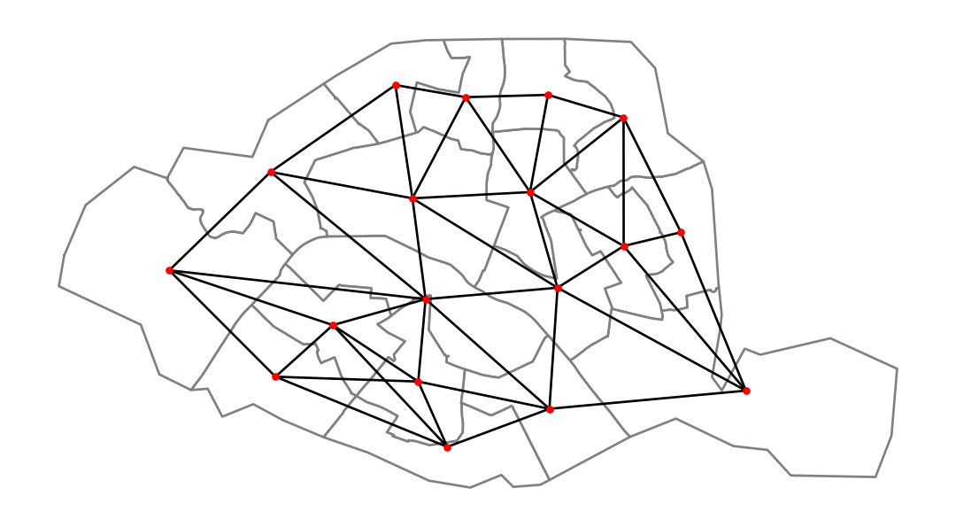

W.neighbors

{'7506': ['7515', '7508', '7516', '7505', '7507'],
 '7505': ['7501', '7517', '7516', '7506', '7518', '7507'],
 '7502': ['7511', '7501', '7512', '7514', '7509', '7504', '7507'],
 '7501': ['7502', '7504', '7503', '7505', '7518', '7507'],
 '7504': ['7502', '7501', '7503', '7514'],
 '7517': ['7516', '7505', '7518'],
 '7512': ['7502', '7511', '7514', '7510', '7513'],
 '7515': ['7508', '7516', '7506'],
 '7511': ['7502', '7512', '7509', '7510', '7513'],
 '7513': ['7511', '7510', '7512', '7514'],
 '7508': ['7509', '7507', '7506', '7515'],
 '7507': ['7502', '7501', '7505', '7508', '7509', '7506'],
 '7503': ['7501', '7504', '7518'],
 '7516': ['7505', '7517', '7506', '7515'],
 '7518': ['7501', '7517', '7505', '7503'],
 '7514': ['7502', '7504', '7513', '7512'],
 '7510': ['7511', '7509', '7513', '7512'],
 '7509': ['7502', '7511', '7508', '7510', '7507']}

W.weights

{'7506': [1.0, 1.0, 1.0, 1.0, 1.0],
 '7505': [1.0, 1.0, 1.0, 1.0, 1.0, 1.0],
 '7502': [1.0, 1.0, 1.0, 1.0, 1.0, 1.0, 1.0],
 '7501': [1.0, 1.0, 1.0, 1.0, 1.0, 1.0],
 '7504': [1.0, 1.0, 1.0, 1.0],
 '7517': [1.0, 1.0, 1.0],
 '7512': [1.0, 1.0, 1.0, 1.0, 1.0],
 '7515': [1.0, 1.0, 1.0],
 '7511': [1.0, 1.0, 1.0, 1.0, 1.0],
 '7513': [1.0, 1.0, 1.0, 1.0],
 '7508': [1.0, 1.0, 1.0, 1.0],
 '7507': [1.0, 1.0, 1.0, 1.0, 1.0, 1.0],
 '7503': [1.0, 1.0, 1.0],
 '7516': [1.0, 1.0, 1.0, 1.0],
 '7518': [1.0, 1.0, 1.0, 1.0],
 '7514': [1.0, 1.0, 1.0, 1.0],
 '7510': [1.0, 1.0, 1.0, 1.0],
 '7509': [1.0, 1.0, 1.0, 1.0, 1.0]}

Adjacency matrix

pd.DataFrame(*W.full()).astype(int)

	0	1	2	3	4	5	6	7	8	9	10	11	12	13	14	15	16	17
7506	0	1	0	0	0	0	0	1	0	0	1	1	0	1	0	0	0	0
7505	1	0	0	1	0	1	0	0	0	0	0	1	0	1	1	0	0	0
7502	0	0	0	1	1	0	1	0	1	0	0	1	0	0	0	1	0	1
7501	0	1	1	0	1	0	0	0	0	0	0	1	1	0	1	0	0	0
7504	0	0	1	1	0	0	0	0	0	0	0	0	1	0	0	1	0	0
7517	0	1	0	0	0	0	0	0	0	0	0	0	0	1	1	0	0	0
7512	0	0	1	0	0	0	0	0	1	1	0	0	0	0	0	1	1	0
7515	1	0	0	0	0	0	0	0	0	0	1	0	0	1	0	0	0	0
7511	0	0	1	0	0	0	1	0	0	1	0	0	0	0	0	0	1	1
7513	0	0	0	0	0	0	1	0	1	0	0	0	0	0	0	1	1	0
7508	1	0	0	0	0	0	0	1	0	0	0	1	0	0	0	0	0	1
7507	1	1	1	1	0	0	0	0	0	0	1	0	0	0	0	0	0	1
7503	0	0	0	1	1	0	0	0	0	0	0	0	0	0	1	0	0	0
7516	1	1	0	0	0	1	0	1	0	0	0	0	0	0	0	0	0	0
7518	0	1	0	1	0	1	0	0	0	0	0	0	1	0	0	0	0	0
7514	0	0	1	0	1	0	1	0	0	1	0	0	0	0	0	0	0	0
7510	0	0	0	0	0	0	1	0	1	1	0	0	0	0	0	0	0	1
7509	0	0	1	0	0	0	0	0	1	0	1	1	0	0	0	0	1	0

Note that we went from geometries to a matrix, which we can work with using usual linear algebra tools

W.cardinalities

{'7506': 5,
 '7505': 6,
 '7502': 7,
 '7501': 6,
 '7504': 4,
 '7517': 3,
 '7512': 5,
 '7515': 3,
 '7511': 5,
 '7513': 4,
 '7508': 4,
 '7507': 6,
 '7503': 3,
 '7516': 4,
 '7518': 4,
 '7514': 4,
 '7510': 4,
 '7509': 5}

W.transform = "R"
pd.DataFrame(*W.full())

	0	1	2	3	4	5	6	7	8	9	10	11	12	13	14	15	16	17
7506	0.000000	0.200000	0.000000	0.000000	0.000000	0.000000	0.000000	0.20	0.000000	0.00	0.200000	0.200000	0.000000	0.200000	0.000000	0.000000	0.00	0.000000
7505	0.166667	0.000000	0.000000	0.166667	0.000000	0.166667	0.000000	0.00	0.000000	0.00	0.000000	0.166667	0.000000	0.166667	0.166667	0.000000	0.00	0.000000
7502	0.000000	0.000000	0.000000	0.142857	0.142857	0.000000	0.142857	0.00	0.142857	0.00	0.000000	0.142857	0.000000	0.000000	0.000000	0.142857	0.00	0.142857
7501	0.000000	0.166667	0.166667	0.000000	0.166667	0.000000	0.000000	0.00	0.000000	0.00	0.000000	0.166667	0.166667	0.000000	0.166667	0.000000	0.00	0.000000
7504	0.000000	0.000000	0.250000	0.250000	0.000000	0.000000	0.000000	0.00	0.000000	0.00	0.000000	0.000000	0.250000	0.000000	0.000000	0.250000	0.00	0.000000
7517	0.000000	0.333333	0.000000	0.000000	0.000000	0.000000	0.000000	0.00	0.000000	0.00	0.000000	0.000000	0.000000	0.333333	0.333333	0.000000	0.00	0.000000
7512	0.000000	0.000000	0.200000	0.000000	0.000000	0.000000	0.000000	0.00	0.200000	0.20	0.000000	0.000000	0.000000	0.000000	0.000000	0.200000	0.20	0.000000
7515	0.333333	0.000000	0.000000	0.000000	0.000000	0.000000	0.000000	0.00	0.000000	0.00	0.333333	0.000000	0.000000	0.333333	0.000000	0.000000	0.00	0.000000
7511	0.000000	0.000000	0.200000	0.000000	0.000000	0.000000	0.200000	0.00	0.000000	0.20	0.000000	0.000000	0.000000	0.000000	0.000000	0.000000	0.20	0.200000
7513	0.000000	0.000000	0.000000	0.000000	0.000000	0.000000	0.250000	0.00	0.250000	0.00	0.000000	0.000000	0.000000	0.000000	0.000000	0.250000	0.25	0.000000
7508	0.250000	0.000000	0.000000	0.000000	0.000000	0.000000	0.000000	0.25	0.000000	0.00	0.000000	0.250000	0.000000	0.000000	0.000000	0.000000	0.00	0.250000
7507	0.166667	0.166667	0.166667	0.166667	0.000000	0.000000	0.000000	0.00	0.000000	0.00	0.166667	0.000000	0.000000	0.000000	0.000000	0.000000	0.00	0.166667
7503	0.000000	0.000000	0.000000	0.333333	0.333333	0.000000	0.000000	0.00	0.000000	0.00	0.000000	0.000000	0.000000	0.000000	0.333333	0.000000	0.00	0.000000
7516	0.250000	0.250000	0.000000	0.000000	0.000000	0.250000	0.000000	0.25	0.000000	0.00	0.000000	0.000000	0.000000	0.000000	0.000000	0.000000	0.00	0.000000
7518	0.000000	0.250000	0.000000	0.250000	0.000000	0.250000	0.000000	0.00	0.000000	0.00	0.000000	0.000000	0.250000	0.000000	0.000000	0.000000	0.00	0.000000
7514	0.000000	0.000000	0.250000	0.000000	0.250000	0.000000	0.250000	0.00	0.000000	0.25	0.000000	0.000000	0.000000	0.000000	0.000000	0.000000	0.00	0.000000
7510	0.000000	0.000000	0.000000	0.000000	0.000000	0.000000	0.250000	0.00	0.250000	0.25	0.000000	0.000000	0.000000	0.000000	0.000000	0.000000	0.00	0.250000
7509	0.000000	0.000000	0.200000	0.000000	0.000000	0.000000	0.000000	0.00	0.200000	0.00	0.200000	0.200000	0.000000	0.000000	0.000000	0.000000	0.20	0.000000

pd.Series(W.cardinalities).plot.hist(color="k")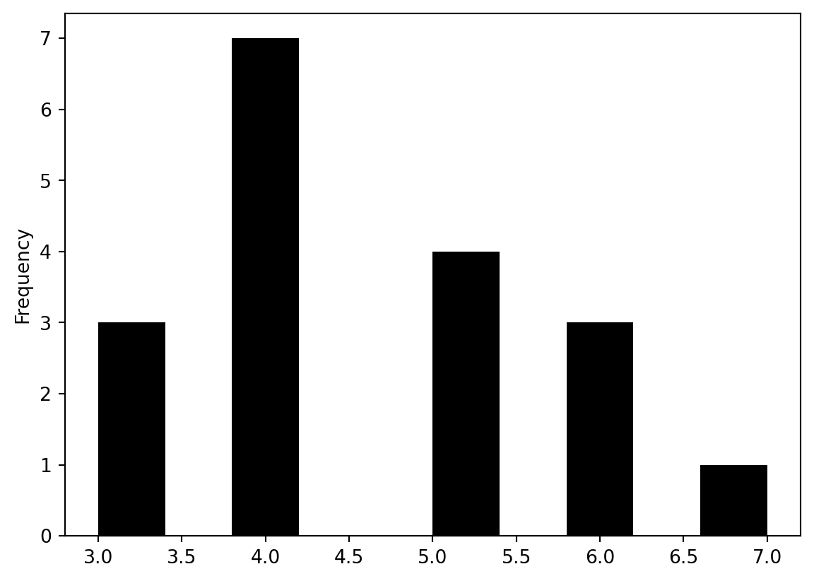

Other possible definition of weights using kernels

W = weights.distance.Kernel.from_dataframe(paris, function = "gaussian")

pd.DataFrame(*W.full())

	0	1	2	3	4	5	6	7	8	9	10	11	12	13	14	15	16	17
52	0.398942	0.338931	0.000000	0.000000	0.000000	0.267739	0.000000	0.380092	0.000000	0.000000	0.241971	0.366320	0.000000	0.316847	0.000000	0.000000	0.000000	0.255290
53	0.338931	0.398942	0.291999	0.328731	0.000000	0.348119	0.000000	0.283863	0.000000	0.000000	0.000000	0.347477	0.264008	0.326715	0.332084	0.000000	0.000000	0.000000
55	0.000000	0.291999	0.398942	0.345396	0.000000	0.000000	0.350514	0.000000	0.362621	0.267876	0.000000	0.312283	0.000000	0.000000	0.000000	0.000000	0.292319	0.272336
56	0.000000	0.328731	0.345396	0.398942	0.298303	0.265964	0.291857	0.000000	0.249691	0.000000	0.000000	0.265977	0.332224	0.000000	0.332484	0.000000	0.000000	0.000000
57	0.000000	0.000000	0.000000	0.298303	0.398942	0.000000	0.272444	0.000000	0.000000	0.000000	0.000000	0.000000	0.288869	0.000000	0.000000	0.302015	0.000000	0.000000
58	0.267739	0.348119	0.000000	0.265964	0.000000	0.398942	0.000000	0.000000	0.000000	0.000000	0.000000	0.000000	0.287942	0.365686	0.362977	0.000000	0.000000	0.000000
59	0.000000	0.000000	0.350514	0.291857	0.272444	0.000000	0.398942	0.000000	0.344688	0.367152	0.000000	0.000000	0.000000	0.000000	0.000000	0.263290	0.270262	0.000000
60	0.380092	0.283863	0.000000	0.000000	0.000000	0.000000	0.000000	0.398942	0.000000	0.000000	0.265076	0.308999	0.000000	0.317139	0.000000	0.000000	0.000000	0.000000
61	0.000000	0.000000	0.362621	0.249691	0.000000	0.000000	0.344688	0.000000	0.398942	0.300098	0.000000	0.269137	0.000000	0.000000	0.000000	0.000000	0.371497	0.310528
74	0.000000	0.000000	0.267876	0.000000	0.000000	0.000000	0.367152	0.000000	0.300098	0.398942	0.000000	0.000000	0.000000	0.000000	0.000000	0.291013	0.246770	0.000000
289	0.241971	0.000000	0.000000	0.000000	0.000000	0.000000	0.000000	0.265076	0.000000	0.000000	0.398942	0.000000	0.000000	0.000000	0.000000	0.000000	0.000000	0.000000
290	0.366320	0.347477	0.312283	0.265977	0.000000	0.000000	0.000000	0.308999	0.269137	0.000000	0.000000	0.398942	0.000000	0.250599	0.000000	0.000000	0.000000	0.324895
291	0.000000	0.264008	0.000000	0.332224	0.288869	0.287942	0.000000	0.000000	0.000000	0.000000	0.000000	0.000000	0.398942	0.000000	0.371598	0.000000	0.000000	0.000000
292	0.316847	0.326715	0.000000	0.000000	0.000000	0.365686	0.000000	0.317139	0.000000	0.000000	0.000000	0.250599	0.000000	0.398942	0.280075	0.000000	0.000000	0.000000
293	0.000000	0.332084	0.000000	0.332484	0.000000	0.362977	0.000000	0.000000	0.000000	0.000000	0.000000	0.000000	0.371598	0.280075	0.398942	0.000000	0.000000	0.000000
294	0.000000	0.000000	0.000000	0.000000	0.302015	0.000000	0.263290	0.000000	0.000000	0.291013	0.000000	0.000000	0.000000	0.000000	0.000000	0.398942	0.000000	0.000000
295	0.000000	0.000000	0.292319	0.000000	0.000000	0.000000	0.270262	0.000000	0.371497	0.246770	0.000000	0.000000	0.000000	0.000000	0.000000	0.000000	0.398942	0.337942
296	0.255290	0.000000	0.272336	0.000000	0.000000	0.000000	0.000000	0.000000	0.310528	0.000000	0.000000	0.324895	0.000000	0.000000	0.000000	0.000000	0.337942	0.398942

full_matrix, ids = W.full()
paris.assign(weight_0 = full_matrix[0]).plot("weight_0", cmap="Reds")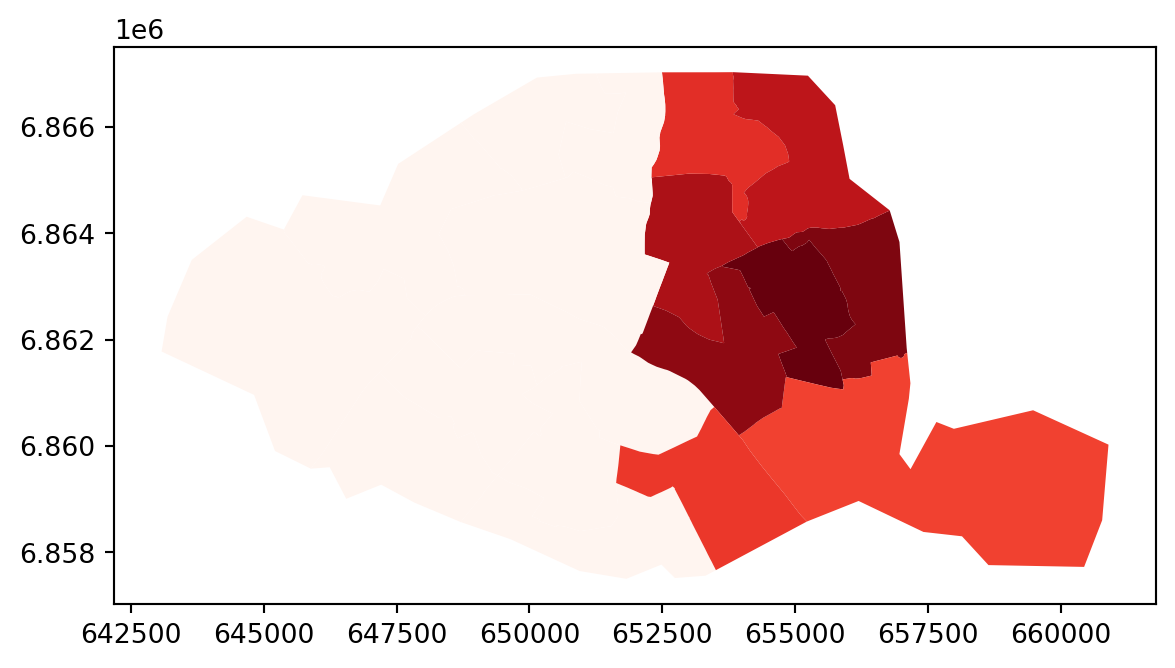

W = weights.distance.Kernel.from_dataframe(paris, function = "triangular", k=15)

full_matrix, ids = W.full()
paris.assign(weight_0 = full_matrix[0]).plot("weight_0", cmap="Reds")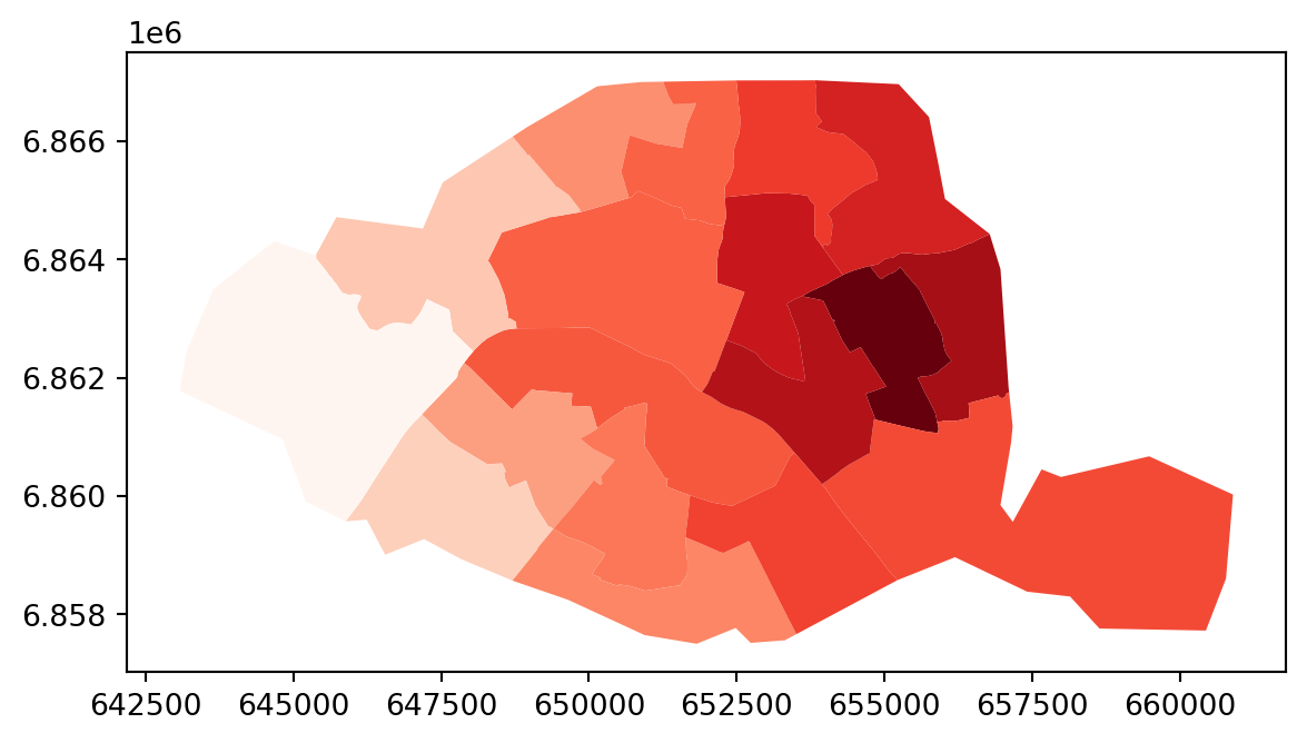

Type	Description	Use Case
Queen Contiguity	Neighbors share edge OR vertex	Polygons (regions)
Rook Contiguity	Neighbors share edge only	Grid data
K-Nearest Neighbors	K closest observations	Point data
Distance Band	All within threshold distance	Point data
Kernel	Distance-weighted	Smooth spatial effects

Practice

• Take the whole constituencies geoDataFrame

  • build the contiguity.Queen weights matrix
  • What is the distribution of the number of neighbours?
  • Which constituencies have the most neighbours?
  • What are the neighbours of constituency 7513?

# TODO

W = weights.contiguity.Queen.from_dataframe(constituencies, idVariable = "id_circo")

pd.Series(W.cardinalities).plot.hist(color="k")

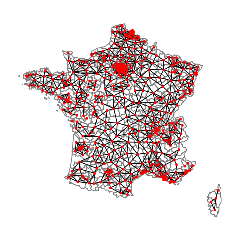
centroids = np.column_stack((constituencies.centroid.x, constituencies.centroid.y))
graph = W.to_networkx()
positions = dict(zip(graph.nodes, centroids))

# plot with a nice basemap
ax = constituencies.plot(linewidth=1, edgecolor="grey", facecolor="white")
nx.draw(graph, positions, ax=ax, node_size=5, node_color="r")
plt.show()

W.neighbors.get('7801')
{z for z in W.cardinalities if W.cardinalities[z] == 9}

/tmp/ipykernel_26467/196323581.py:3: FutureWarning: `idVariable` is deprecated and will be removed in future. Use `ids` instead.
  W = weights.contiguity.Queen.from_dataframe(constituencies, idVariable = "id_circo")
/opt/python/lib/python3.13/site-packages/libpysal/weights/contiguity.py:347: UserWarning: The weights matrix is not fully connected: 
 There are 11 disconnected components.
 There are 5 islands with ids: 4405, 7902, 0602, 0605, 1701.
  W.__init__(self, neighbors, ids=ids, **kw)
/tmp/ipykernel_26467/196323581.py:7: UserWarning: Geometry is in a geographic CRS. Results from 'centroid' are likely incorrect. Use 'GeoSeries.to_crs()' to re-project geometries to a projected CRS before this operation.

  centroids = np.column_stack((constituencies.centroid.x, constituencies.centroid.y))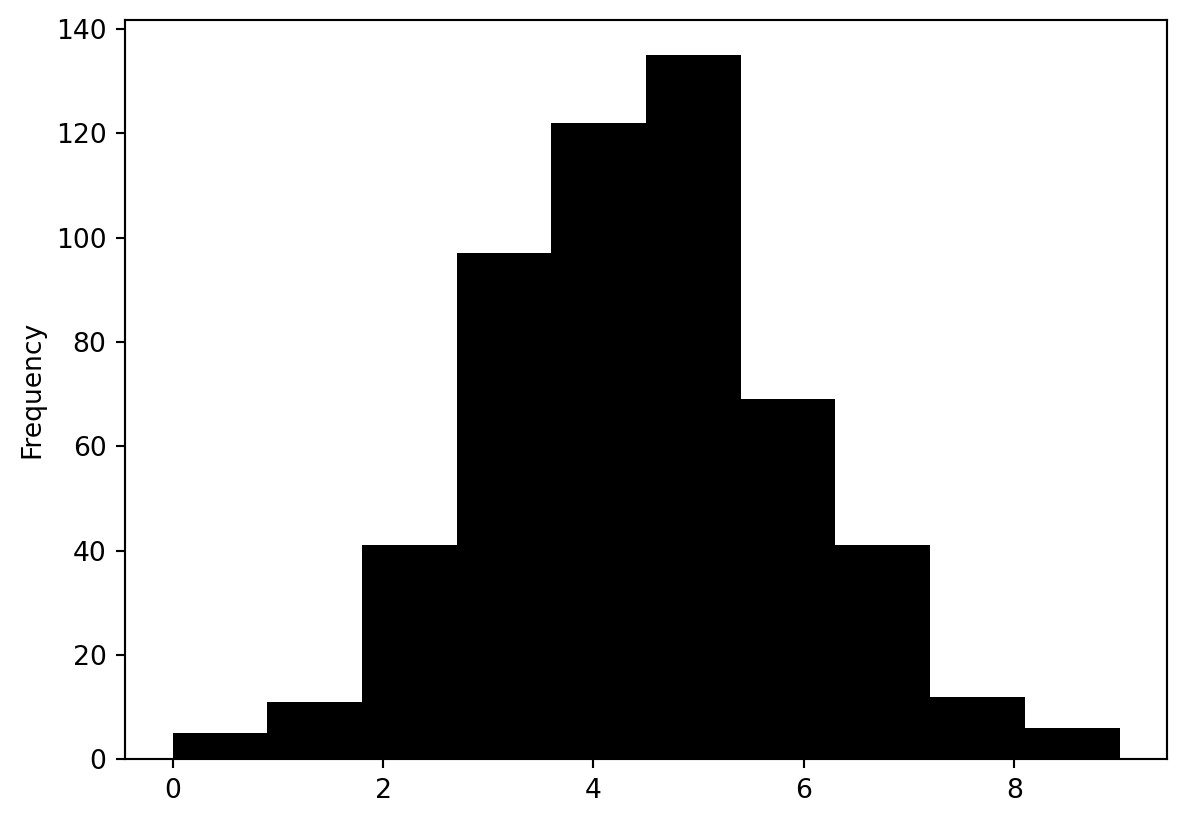

{'0205', '5704', '5802', '6201', '7602', '8004'}

Spatial autocorrelation

constituencies.plot("vote_share_rn", cmap="Greys")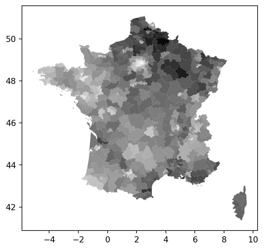

Global autocorrelation

How does the vote share of any given constituency relate to the constituencies of its neighbouring constituencies?

• are “high” vote constituencies close to “high” vote constituencies? “low” to “low”?
• or “high” to “low” and “low” to “high”?
• or pure randomness?

W = weights.contiguity.Queen.from_dataframe(constituencies, ids = "id_circo")
W.transform = "R" # row standardization: rows sum to 1

('WARNING: ', '4405', ' is an island (no neighbors)')
('WARNING: ', '7902', ' is an island (no neighbors)')
('WARNING: ', '0602', ' is an island (no neighbors)')
('WARNING: ', '0605', ' is an island (no neighbors)')
('WARNING: ', '1701', ' is an island (no neighbors)')

/opt/python/lib/python3.13/site-packages/libpysal/weights/contiguity.py:347: UserWarning: The weights matrix is not fully connected: 
 There are 11 disconnected components.
 There are 5 islands with ids: 4405, 7902, 0602, 0605, 1701.
  W.__init__(self, neighbors, ids=ids, **kw)

Spatial lag operator (analogous to time lag operator in time series):

\(X_{lag} = WX\)

\(X_{lag} = \sum_{i} w_i x_i\)

If W is row normalized, this is a weighted averages of neighbor values using the spatial weights

We can now reframe the spatial autocorrelation as:

\(Corr(X, X_{lag})\)

constituencies["lagged_vote_share_rn"] = weights.spatial_lag.lag_spatial(W, constituencies["vote_share_rn"])

constituencies[["vote_share_rn", "lagged_vote_share_rn"]]

	vote_share_rn	lagged_vote_share_rn
0	20.41	25.694000
1	14.39	25.033333
2	38.43	37.555000
3	28.41	28.304000
4	27.67	22.557500
...	...	...
534	29.44	34.086667
535	38.50	39.245000
536	38.62	35.733750
537	32.02	36.588000
538	32.56	30.520000

539 rows × 2 columns

constituencies.plot("lagged_vote_share_rn", cmap="Greys")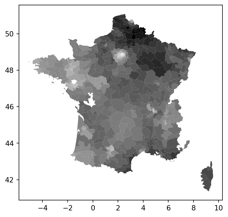

constituencies["vote_share_rn_standardized"] = constituencies["vote_share_rn"] - constituencies["vote_share_rn"].mean()
constituencies["lagged_vote_share_rn_standardized"] = weights.lag_spatial(W, constituencies["vote_share_rn_standardized"])

fig, ax = plt.subplots(figsize=(9, 9))
ax.scatter(constituencies["vote_share_rn_standardized"], constituencies["lagged_vote_share_rn_standardized"])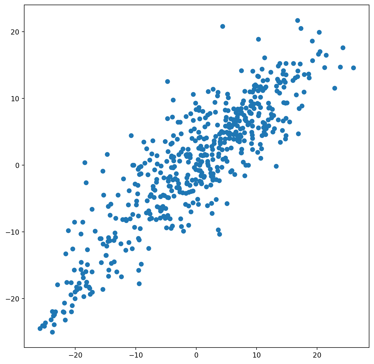

constituencies[["vote_share_rn", "lagged_vote_share_rn"]].corr()

	vote_share_rn	lagged_vote_share_rn
vote_share_rn	1.00000	0.83766
lagged_vote_share_rn	0.83766	1.00000

Similar concept with good statistical properties: Moran’s I

\(I = \frac{n \sum_i \sum_j w_{ij}(Y_i - \bar Y)(Y_j - \bar Y)} {(\sum_{i \neq j} w_{ij}) \sum_i (Y_i - \bar Y)^2} = \frac{n}{\sum_{i \neq j} w_{ij}} \frac{\sum_i \sum_j w_{ij} z_i z_j}{\sum_i z_i^2}\)

moran = esda.moran.Moran(constituencies["vote_share_rn"], W)
moran.I

np.float64(0.7794561095576024)

moran.p_sim

np.float64(0.001)

plot_moran(moran)

(<Figure size 960x384 with 2 Axes>,
 array([<Axes: title={'center': 'Reference Distribution'}, xlabel='Moran I: 0.78', ylabel='Density'>,
        <Axes: title={'center': 'Moran Scatterplot (0.78)'}, xlabel='Attribute', ylabel='Spatial Lag'>],
       dtype=object))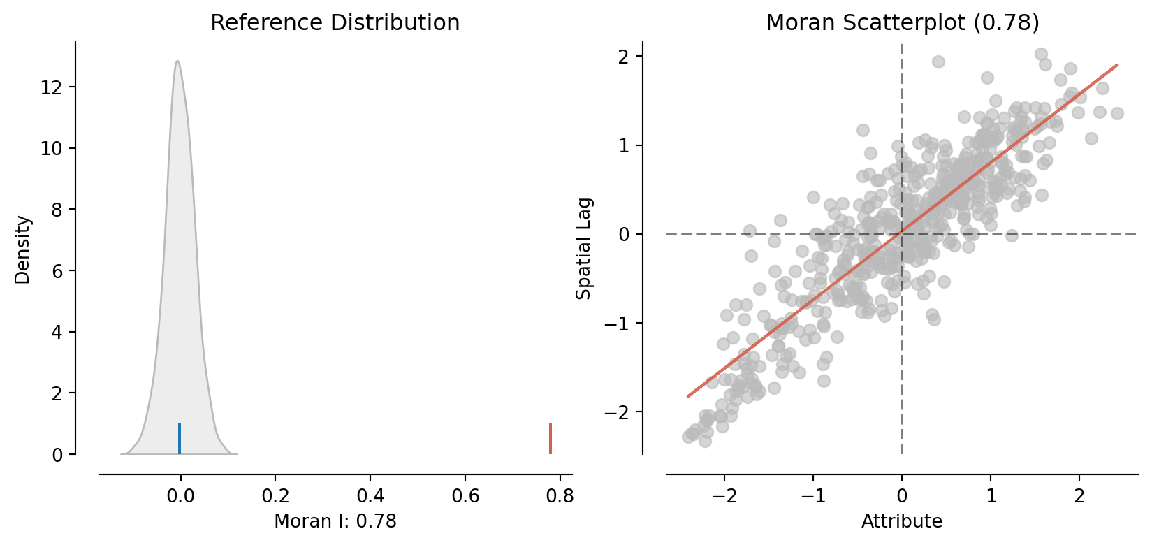

Practice

• Plot a chloropleth map of D9_diff (9-th decile income) (cast D9 as a float first)
• Compute its spatially lagged value
• Plot D9 and its spatially lagged value: what is the relationship between the two?
• Compute Moran’s I

moran = esda.moran.Moran(constituencies["D9_diff"].astype(float), W)
plot_moran(moran)

(<Figure size 960x384 with 2 Axes>,
 array([<Axes: title={'center': 'Reference Distribution'}, xlabel='Moran I: 0.75', ylabel='Density'>,
        <Axes: title={'center': 'Moran Scatterplot (0.75)'}, xlabel='Attribute', ylabel='Spatial Lag'>],
       dtype=object))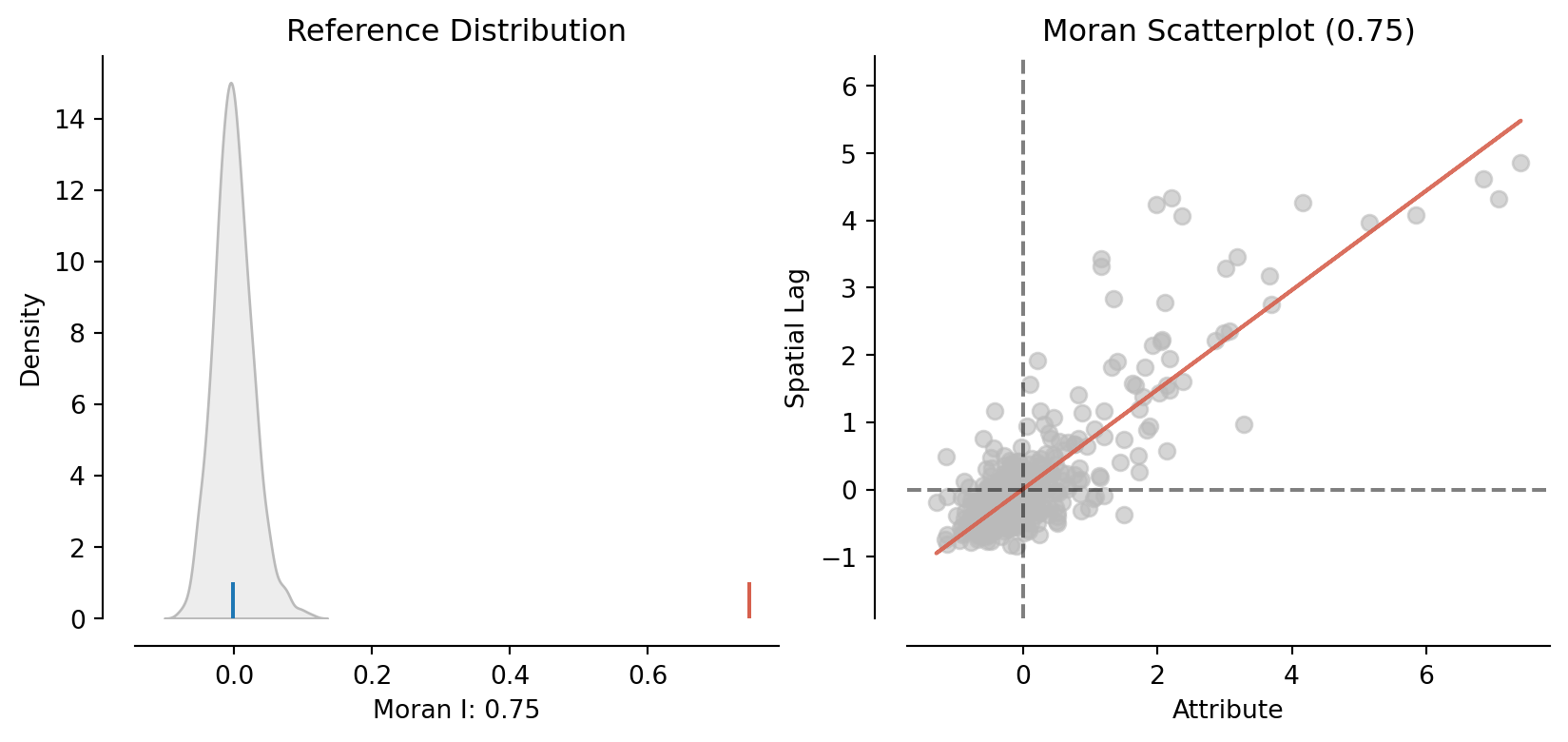

constituencies.plot("D9_diff", cmap="Reds")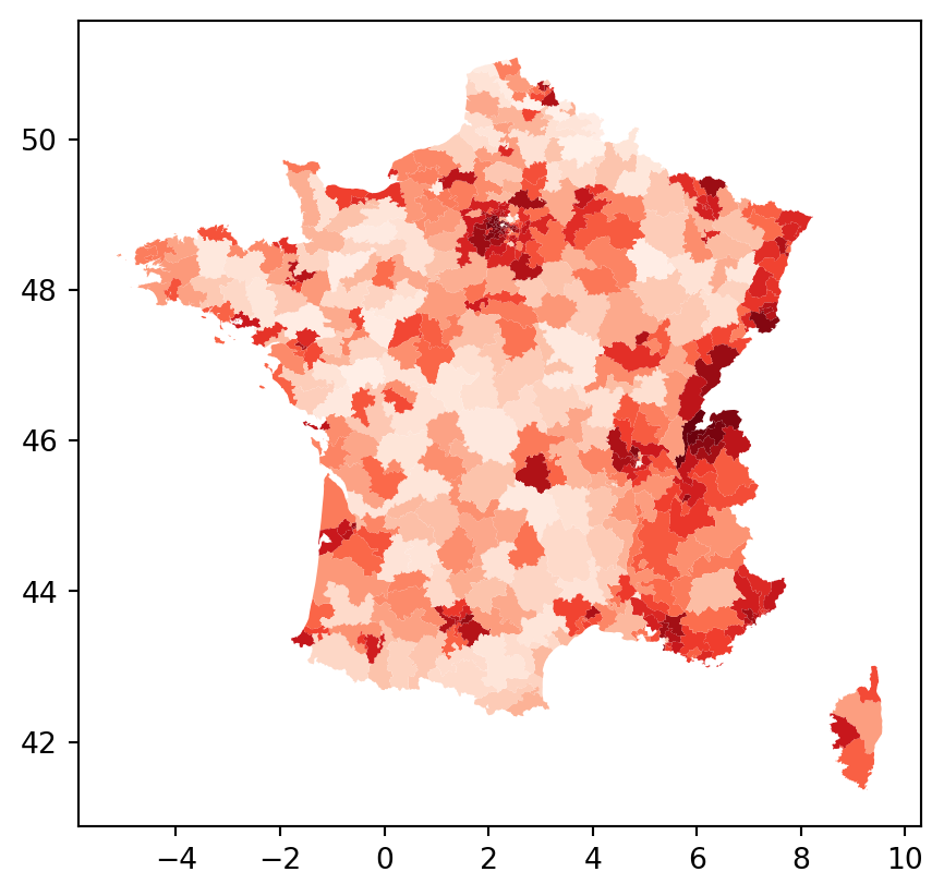

Local autocorrelation

One Local Indicator of Spatial Association (LISA) is local Moran’s I: global Moran’s I, expect we don’t sum over the i’s

\(I_i = \frac{n}{\sum_{i} z_{i}^2} z_{i} \sum_{j} w_{i,j}z_{j}\)

lisa = esda.moran.Moran_Local(constituencies["vote_share_rn"], W)
lisa.Is

/opt/python/lib/python3.13/site-packages/esda/moran.py:1350: RuntimeWarning: invalid value encountered in divide
  self.z_sim = (self.Is - self.EI_sim) / self.seI_sim

array([ 5.79424752e-01,  9.88925307e-01,  3.48507625e-01,  9.35026207e-02,
        3.12888167e-01,  8.24897842e-01, -1.25263747e-01,  9.06920602e-01,
        9.26783838e-01,  1.38754803e+00,  1.40285754e+00, -1.05035562e-02,
        8.19739723e-01,  6.11477304e-02,  2.77357751e-02,  1.79380083e+00,
        7.42958401e-02,  7.13910752e-01, -1.98169549e-02,  1.37322264e-01,
        1.63967005e-01, -2.47265333e-02, -0.00000000e+00,  3.23873650e-01,
        2.48517940e+00,  2.75701188e+00,  1.70449698e+00, -1.58206529e-01,
       -8.14702695e-02,  1.18986244e-01,  2.53174694e-01, -1.02672730e-01,
       -1.54155086e-02,  2.58171656e-02,  2.68546977e-02,  3.43235069e-01,
        2.47691054e-01,  2.96179373e-01,  1.36454129e+00,  1.44775693e+00,
        9.42053418e-02,  4.02394253e-02,  1.97047060e+00,  1.13667614e-01,
        2.52146643e+00,  3.56473156e+00,  1.14930115e+00,  1.17335681e+00,
        3.13413875e+00,  2.83922544e+00,  9.60659579e-02,  2.58408250e+00,
        5.30615784e+00,  5.48890188e+00,  3.65903257e-01,  4.55052128e+00,
        4.87068166e+00,  3.74737822e+00,  5.16031545e+00,  4.19224185e+00,
        4.62637617e+00,  4.52929475e+00,  1.59978600e+00,  1.17804244e+00,
        2.91669832e+00,  5.38406562e-01,  5.00634563e-01,  3.15589980e+00,
        1.69755895e+00,  8.55677834e-01,  5.93958713e-01,  1.76636973e+00,
        3.29483049e+00,  3.02526901e+00,  3.93050870e+00, -5.20289444e-01,
        2.25870942e+00,  1.08669322e+00, -4.06522442e-02,  3.09635879e+00,
        3.29975029e-02,  1.70319198e-01,  1.57884791e+00,  1.18592404e+00,
        3.45042594e-01,  2.51850089e-01,  7.01140706e-01,  1.27575648e-02,
        4.56957189e-01,  8.21536916e-01,  2.18248678e-03,  3.42894955e-01,
        1.68311913e+00,  2.39812304e+00,  1.49995325e+00, -4.02316305e-02,
        2.22271167e+00,  9.89781427e-01,  2.90597784e-01,  1.48844443e+00,
        2.06554395e-01,  2.58297934e-01, -3.04278903e-01,  9.05335362e-01,
       -1.62553252e-01,  1.30026941e+00, -4.15726652e-01, -2.29787771e-01,
        7.00528600e-01,  1.10907471e-01,  2.73189899e+00,  3.25895727e+00,
        1.45217883e+00,  2.49283314e+00,  2.81186968e+00,  3.30151349e+00,
        1.74288049e+00,  2.11219195e-01,  1.14398828e+00,  8.28083086e-01,
        9.40890363e-01,  1.44428172e-01, -9.57537177e-02,  7.79064501e-01,
        5.11745666e-01, -7.69226002e-02,  3.16159333e-01,  2.94033218e-02,
        9.67503051e-01,  5.05823108e-01,  2.83858330e-01,  5.29909648e-01,
       -2.06094261e-02,  1.82628202e+00, -4.24077887e-02, -6.55306653e-02,
        8.50001656e-01,  1.33244086e+00,  1.18647672e+00,  2.17784018e-01,
       -6.12800832e-02, -1.46183761e-01,  2.97139022e+00,  3.15803899e+00,
        2.84935962e+00,  4.09514123e-01,  5.10286548e-01,  1.93541422e+00,
        1.98553165e-01,  4.20891368e-02,  5.45127823e-02,  1.92332055e-01,
        1.21613170e-01,  1.05657155e-01,  4.20208673e-01,  2.81538142e-01,
        5.12524981e-01, -2.46203720e-02,  4.15022366e-01, -1.08526558e-01,
        3.06288642e-01,  3.92813147e-01,  4.78513586e-01,  6.90631438e-02,
       -4.79518589e-02,  3.60153107e-01,  1.82705316e-01,  3.61782559e-01,
        6.15019900e-01,  3.70142998e-01,  9.23386958e-02,  9.11971151e-01,
        8.70520843e-01, -3.24646581e-01,  4.73437257e-01,  1.46883204e+00,
        2.61843871e+00,  2.10688366e-01, -8.26927295e-02,  1.47534520e-02,
        4.56830275e-02,  1.04303287e-01, -1.82945744e-02,  6.31108292e-02,
       -4.68355690e-02, -1.33216478e-02,  1.77183392e+00,  1.74745389e+00,
        1.29032517e+00, -4.28227904e-03, -1.82165813e-02,  1.91001878e-01,
        3.97848456e-01,  3.08249939e+00, -1.45798882e-01,  6.11845203e-01,
        4.50029155e-01,  9.09703204e-02,  2.84924795e-01,  8.03747041e-02,
        3.20169942e+00,  2.12213150e+00,  7.85002532e-01,  1.35700462e+00,
        1.89441254e-01,  1.48867165e+00,  6.70957869e-01,  1.24973197e+00,
        1.60965093e-02,  3.42593815e-01, -2.61759140e-01,  1.34615420e+00,
        9.91455859e-01,  1.02690628e+00,  5.48627965e-01,  4.42149186e-02,
       -5.32605896e-03,  2.94146049e+00,  2.10785040e+00,  1.07367973e+00,
        5.49774940e-01,  6.54111344e-01,  4.17327226e-01,  3.63750394e-02,
        1.79106348e+00,  1.38454125e-01,  5.12039567e-01,  2.24170593e-02,
        4.70411928e-01,  1.79617381e+00,  2.74923609e+00, -1.69456124e-01,
        2.06975639e-03,  5.11287271e-01,  0.00000000e+00,  4.00348526e-01,
        7.60382047e-01,  9.16355674e-01,  3.02051483e-01,  1.49239988e+00,
        2.64043159e+00, -1.08398642e-01, -2.29259962e-02,  6.91443225e-01,
        8.94204180e-01,  5.96233170e-02,  4.39191849e-04,  2.09330337e+00,
        8.62538231e-01,  7.52011765e-01,  7.60384441e-01,  2.32662712e+00,
        1.30730050e+00,  1.74965880e+00,  3.07252352e+00,  5.78889488e-01,
        1.19555329e-01,  2.31697555e-01,  1.75435856e-02, -2.40264396e-02,
        8.69690967e-02,  3.95275720e-01, -2.77904546e-02,  7.04733298e-02,
        0.00000000e+00, -1.08617828e-01,  5.03257817e-01,  3.07911405e+00,
        7.49271292e-02,  0.00000000e+00,  1.50366792e+00,  3.49201588e+00,
        5.01264555e-01,  1.20186471e-01,  1.82390683e+00,  3.58278633e-01,
        8.31512038e-01, -4.10591594e-02,  1.12098582e+00,  1.21503582e+00,
       -2.61845309e-02,  2.40728786e-01,  8.53187774e-02,  3.17734797e+00,
        5.65084490e-02,  6.42112323e-02,  1.95820083e-01,  6.29224598e-01,
        3.09752510e-01,  3.90199438e+00,  5.11510030e+00,  4.43362601e+00,
        4.81736065e+00,  5.25387720e+00,  3.47789569e+00,  4.17980233e+00,
        4.35436558e+00,  9.75683211e-02,  2.84194535e-01,  1.85856610e+00,
        3.04383619e+00,  2.29180748e+00,  1.51425873e+00,  1.96138499e+00,
        9.18175801e-01,  3.70361284e+00,  2.20047080e+00, -3.44602925e-01,
        3.51415175e+00,  1.25683251e+00,  2.12801095e+00,  1.48043114e+00,
        8.38722592e-02,  2.18100265e-01,  1.83910413e-02,  4.82253023e-01,
        4.49639564e-01,  2.18792083e-01, -6.10555829e-02,  8.42442858e-03,
        4.78527898e-01,  7.98747751e-01,  2.33055823e-02,  3.45017707e-01,
        1.70883960e-01, -1.51897743e-02, -0.00000000e+00,  2.19816571e-01,
        1.13635832e+00,  2.05987422e+00,  1.13695150e-02,  3.62864992e-02,
        5.47745892e-01,  4.74759047e-01,  4.10741648e-01, -3.01369000e-02,
       -8.09462004e-03,  6.13663897e-01, -4.94498333e-02,  7.68270774e-01,
       -1.15930142e-01,  1.07157130e+00,  3.18578686e-01,  2.01039048e-02,
        1.96887363e-01,  3.33692194e-01,  1.43430061e+00,  1.02137669e+00,
        1.51967396e+00,  6.12561440e-01,  4.57202396e-01,  1.02198893e-02,
        8.32518451e-02,  9.17135242e-01,  2.38647724e+00,  5.54203393e-02,
        4.35788239e-02,  6.58410559e-02,  8.47811802e-01,  5.44884396e-01,
        7.05546329e-01,  2.86429117e-01, -4.27529600e-02,  1.17828835e+00,
        2.11222866e-01,  1.53207322e-01, -1.16329928e-02,  5.20705470e-03,
        2.86304601e-01,  1.83217718e-01,  2.76379832e-02, -5.26464959e-02,
       -2.07755015e-02,  7.91113078e-02,  4.85859488e-01,  1.21554960e-01,
        3.21105300e-02,  5.05050623e-02,  1.94524383e-01,  2.22110235e-01,
       -2.47814451e-01, -2.54067786e-02,  2.16612670e-01,  2.91660760e-01,
       -3.03985600e-02,  4.25433990e-01,  1.30570010e-01, -1.68536243e-02,
        3.76561615e-02,  1.83803519e-02,  1.23295473e-02, -1.17269388e-02,
        4.59173805e-03, -2.14560109e-02,  1.59544306e-02,  4.13152118e-03,
        1.01189647e-03,  6.15413191e-01,  2.74615128e-01,  1.70053419e+00,
        2.37449605e-02, -4.02985956e-02,  1.74369137e+00,  5.03138732e-01,
        1.58639175e+00, -1.50879442e-02, -5.15752311e-04,  5.30372146e-03,
       -1.16813444e-01,  6.13136914e-01,  6.92836924e-01,  5.73806851e-01,
       -1.06127496e-01,  1.34865636e-01,  2.69740094e+00,  2.33479995e-01,
       -9.22112576e-03,  1.26329075e-03, -2.52585528e-01,  2.52405101e-01,
        2.14718661e-03,  3.54029743e-01,  6.19330983e-02,  8.24750244e-01,
        2.62205341e-01,  3.63996200e-01,  2.63784660e-01,  8.12508261e-01,
        1.55333662e-01,  6.14627535e-01,  3.75097917e-01,  2.73676585e-01,
        1.08440210e+00,  1.89722181e-01, -6.10932741e-02,  2.53458154e-02,
        4.19547823e-02,  1.98813344e+00,  8.82451051e-01,  5.07341619e-01,
        6.02967390e-02,  8.30283428e-01,  1.20173172e-01,  2.69457937e-01,
       -3.98251622e-02,  1.29369744e-02,  6.01611091e-01, -2.12235934e-02,
        9.97359636e-02,  3.44458059e-02, -2.09903378e-01,  1.70403964e+00,
        1.36669557e+00,  7.10199153e-01, -3.50648693e-02, -1.76394409e-01,
        9.67987453e-03, -2.87070713e-08,  2.28975795e-01,  1.84228683e-01,
        2.34032954e-01,  2.45268843e-01,  2.84829380e-01,  4.84907331e-01,
        1.55813743e-01,  7.64179470e-01,  3.09957578e-01,  1.28960924e+00,
        7.96548779e-01,  1.57967088e+00,  3.25739812e-01,  4.98904341e-01,
        3.73921757e-01,  3.06511387e-02,  1.21472305e+00,  1.55789710e+00,
        6.60601726e-01,  4.64702169e-01, -1.49765826e-01,  8.67988573e-02,
        1.99835938e-02, -2.73940159e-03,  3.46559423e-02, -1.72224335e-02,
        5.48203157e-02,  3.37493794e-01,  9.90672759e-02,  6.45834912e-01,
        7.73266648e-01,  4.64775424e-01, -1.13854918e-02,  3.60500213e-01,
        1.90271251e-01, -7.57584033e-02,  2.91739444e-01, -4.85033794e-02,
        3.41601264e-01, -9.27450200e-03,  1.97961112e+00, -4.46914851e-03,
        1.77118107e-02, -9.86883804e-03,  1.16671751e-01, -4.92884640e-02,
        9.94937072e-02,  1.27462575e+00, -3.62936487e-03,  1.24311111e-01,
        2.47265519e-01, -1.04231823e-02,  2.82315051e+00,  6.14006753e-01,
        9.42654177e-01,  1.17474992e+00, -1.89648058e-02,  1.21860624e-01,
        3.67344069e-01,  2.14970044e-01,  1.19577932e+00,  1.28914042e+00,
        1.49288061e+00,  9.14251674e-01,  1.79476656e-01,  3.29946767e-01,
        9.48627308e-02,  8.55177993e-02,  2.30666555e-01, -5.30234222e-02,
        1.46999038e-01,  4.58705007e-01,  3.52191601e-01,  3.41343557e-02,
       -2.88194629e-01,  3.46731968e-01, -4.67076659e-02,  4.52700954e-01,
        2.47949894e-01,  1.63147628e-02, -8.94117501e-03])

plt.hist(lisa.Is)

(array([165., 189.,  68.,  47.,  17.,  22.,  13.,   6.,   7.,   5.]),
 array([-0.52028944,  0.08062969,  0.68154882,  1.28246795,  1.88338709,
         2.48430622,  3.08522535,  3.68614448,  4.28706361,  4.88798275,
         5.48890188]),
 <BarContainer object of 10 artists>)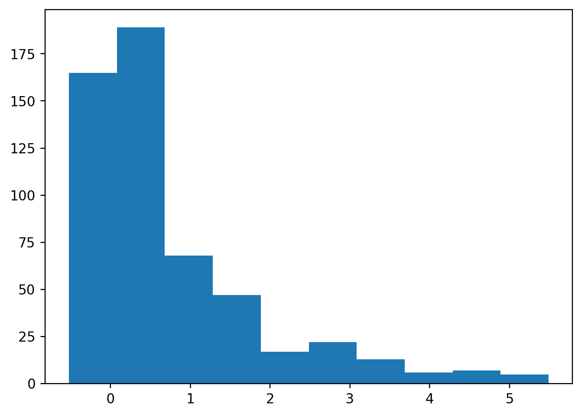

lisa.Is.mean()

np.float64(0.7707928329691234)

constituencies.assign(i=lisa.Is).plot(column="i", cmap = "Reds")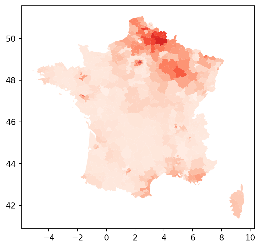

lisa_cluster(lisa, constituencies, p=1)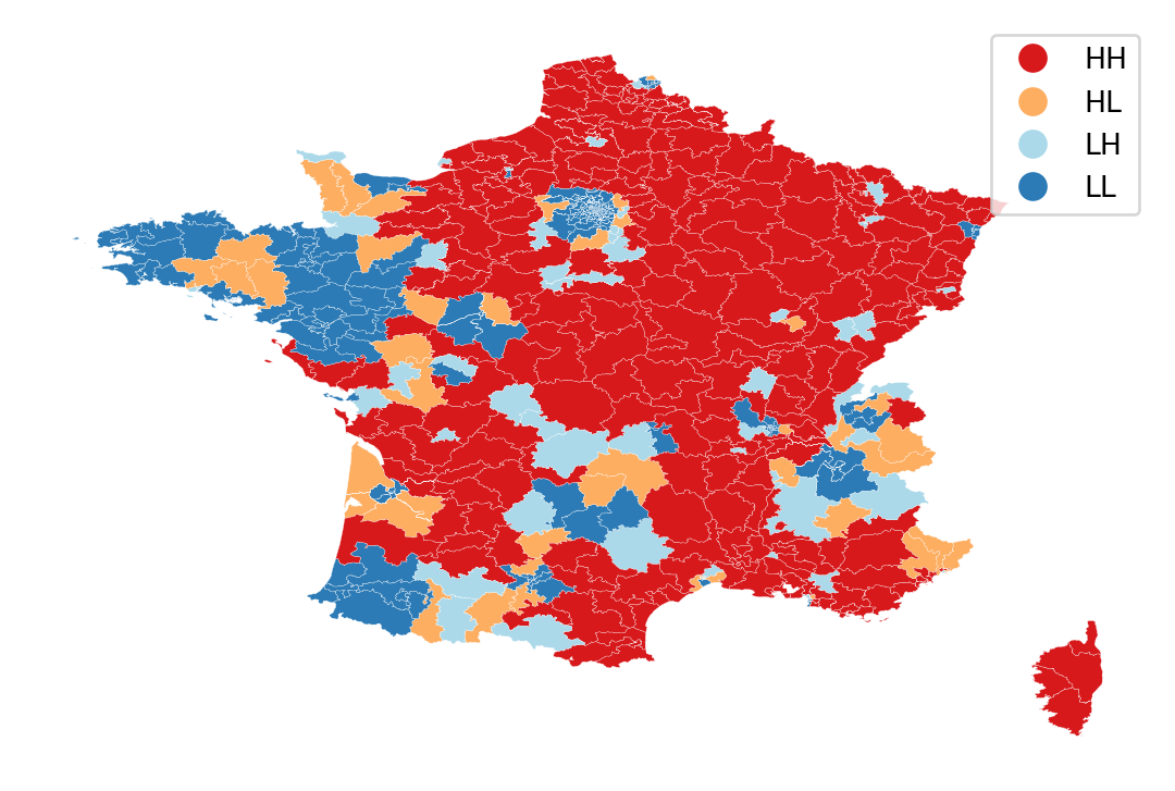

lisa_cluster(lisa, constituencies, p=0.05)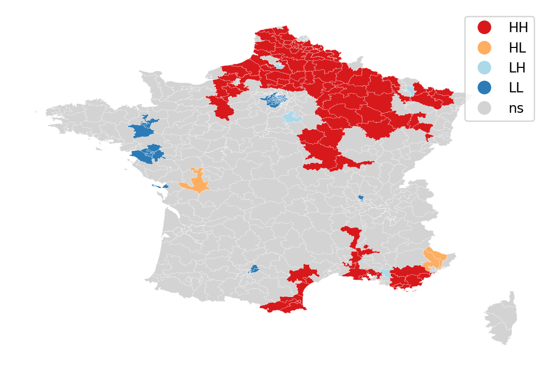

Practice

• Compute local Moran’s I for D1_diff
• Plot the Is, and the LL/HL/LH/HH clusters

Standard geographic regression models

• If the data generating process is explicitly spatial, we want to include geography in the analysis
• If some omitted variables is spatial, resulting errors will be spatial

Let’s see if we can predict/explain vote_share_rn with our explanatory variables

constituencies["D1_diff"] = constituencies["D1_diff"].astype(float)
constituencies["D9_diff"] = constituencies["D9_diff"].astype(float)

ols_model = spreg.OLS(
    constituencies[['vote_share_rn']].values,
    constituencies[['unemployement_rate', 'mean_age', 'D1_diff', 'D9_diff']].values,
    # Dependent variable name
    name_y="vote_share_rn",
    # Independent variable name
    name_x=['unemployement_rate', 'mean_age', 'D1_diff', 'D9_diff'],
)

print(ols_model.summary)

REGRESSION RESULTS
------------------

SUMMARY OF OUTPUT: ORDINARY LEAST SQUARES
------------------------------------------------------------------------------------
Data set            :     unknown
Weights matrix      :        None
Dependent Variable  :vote_share_rn                Number of Observations:         539
Mean dependent var  :     31.6400                Number of Variables   :           5
S.D. dependent var  :     10.7351                Degrees of Freedom    :         534
R-squared           :      0.4494
Adjusted R-squared  :      0.4452
Sum squared residual:     34140.1                F-statistic           :    108.9422
Sigma-square        :      63.933                Prob(F-statistic)     :   7.867e-68
S.E. of regression  :       7.996                Log likelihood        :   -1882.832
Sigma-square ML     :      63.340                Akaike info criterion :    3775.664
S.E of regression ML:      7.9586                Schwarz criterion     :    3797.113

------------------------------------------------------------------------------------
            Variable     Coefficient       Std.Error     t-Statistic     Probability
------------------------------------------------------------------------------------
            CONSTANT       -59.14834        11.61176        -5.09383         0.00000
  unemployement_rate         3.02469         0.53091         5.69717         0.00000
            mean_age         1.36535         0.12838        10.63541         0.00000
             D1_diff         0.00313         0.00050         6.22522         0.00000
             D9_diff        -0.00054         0.00004       -14.03249         0.00000
------------------------------------------------------------------------------------

REGRESSION DIAGNOSTICS
MULTICOLLINEARITY CONDITION NUMBER          86.220

TEST ON NORMALITY OF ERRORS
TEST                             DF        VALUE           PROB
Jarque-Bera                       2          7.609           0.0223

DIAGNOSTICS FOR HETEROSKEDASTICITY
RANDOM COEFFICIENTS
TEST                             DF        VALUE           PROB
Breusch-Pagan test                4         47.549           0.0000
Koenker-Bassett test              4         64.950           0.0000
================================ END OF REPORT =====================================

constituencies.assign(predy=ols_model.predy).plot(column="predy", cmap = "Reds")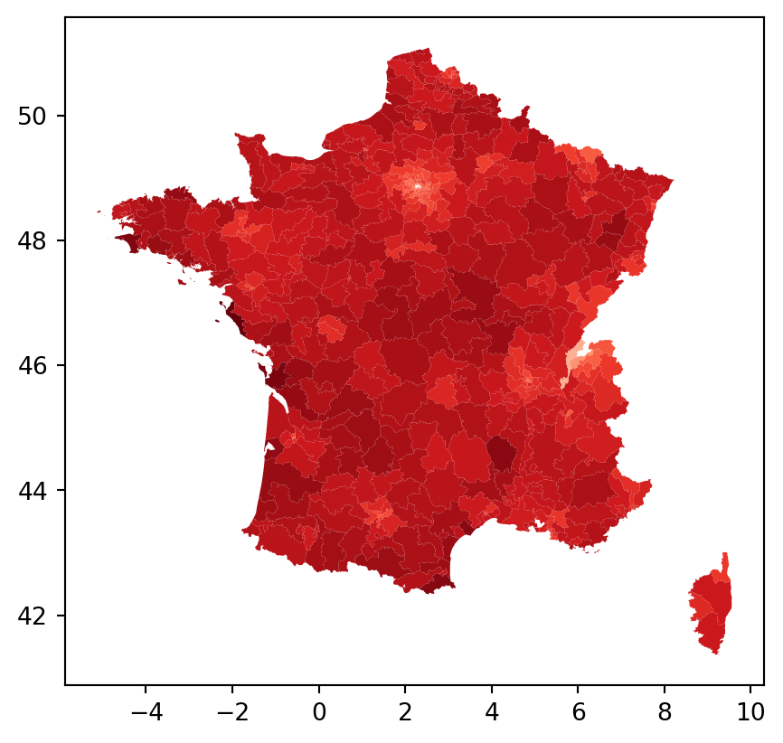

constituencies.assign(u=ols_model.u).plot(column="u", cmap = "seismic", legend = True)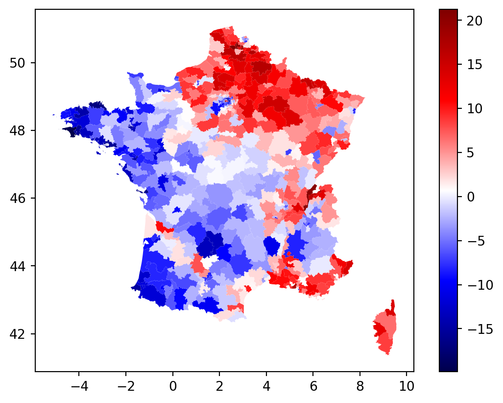

constituencies['u'] = ols_model.u
# constituencies.boxplot(column = ['residuals'], by = "dep", figsize = (20, 5))
constituencies["lagged_u"] = weights.lag_spatial(W, constituencies["u"])

fig, ax = plt.subplots(figsize=(9, 9))
ax.scatter(constituencies["u"], constituencies["lagged_u"])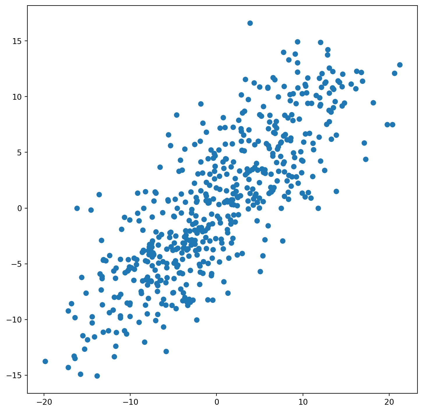

SLX model

Add spatially lagged values as exogenous variables, i.e. \(WX_j\) influence \(Y_i\)

constituencies["lagged_unemployement_rate"] = weights.lag_spatial(W, constituencies["unemployement_rate"])
constituencies["lagged_mean_age"] = weights.lag_spatial(W, constituencies["mean_age"])
constituencies["lagged_D1_diff"] = weights.lag_spatial(W, constituencies["D1_diff"])
constituencies["lagged_D9_diff"] = weights.lag_spatial(W, constituencies["D9_diff"])

variables = ['unemployement_rate', 'mean_age', 'D1_diff', 'D9_diff']
lagged_variables = ["lagged_" + x for x in variables]
all_variables = variables + lagged_variables

slx_model = spreg.OLS(
    constituencies[['vote_share_rn']].values,
    constituencies[all_variables].values,
    # Dependent variable name
    name_y="vote_share_rn",
    # Independent variable name
    name_x=all_variables
)

print(slx_model.summary)

REGRESSION RESULTS
------------------

SUMMARY OF OUTPUT: ORDINARY LEAST SQUARES
------------------------------------------------------------------------------------
Data set            :     unknown
Weights matrix      :        None
Dependent Variable  :vote_share_rn                Number of Observations:         539
Mean dependent var  :     31.6400                Number of Variables   :           9
S.D. dependent var  :     10.7351                Degrees of Freedom    :         530
R-squared           :      0.4732
Adjusted R-squared  :      0.4653
Sum squared residual:     32661.4                F-statistic           :     59.5100
Sigma-square        :      61.625                Prob(F-statistic)     :   5.854e-69
S.E. of regression  :       7.850                Log likelihood        :   -1870.899
Sigma-square ML     :      60.596                Akaike info criterion :    3759.798
S.E of regression ML:      7.7844                Schwarz criterion     :    3798.406

------------------------------------------------------------------------------------
            Variable     Coefficient       Std.Error     t-Statistic     Probability
------------------------------------------------------------------------------------
            CONSTANT       -59.35288        11.79147        -5.03354         0.00000
  unemployement_rate         2.16722         0.58391         3.71157         0.00023
            mean_age         1.30285         0.19924         6.53918         0.00000
             D1_diff         0.00310         0.00062         5.02964         0.00000
             D9_diff        -0.00046         0.00007        -6.09763         0.00000
lagged_unemployement_rate         1.74391         0.50921         3.42472         0.00066
     lagged_mean_age         0.05791         0.19780         0.29279         0.76980
      lagged_D1_diff        -0.00026         0.00060        -0.44086         0.65949
      lagged_D9_diff        -0.00011         0.00009        -1.33309         0.18307
------------------------------------------------------------------------------------

REGRESSION DIAGNOSTICS
MULTICOLLINEARITY CONDITION NUMBER         122.403

TEST ON NORMALITY OF ERRORS
TEST                             DF        VALUE           PROB
Jarque-Bera                       2          3.904           0.1420

DIAGNOSTICS FOR HETEROSKEDASTICITY
RANDOM COEFFICIENTS
TEST                             DF        VALUE           PROB
Breusch-Pagan test                8         83.573           0.0000
Koenker-Bassett test              8        104.473           0.0000
================================ END OF REPORT =====================================

slx_model_2 = spreg.OLS(
    constituencies[['vote_share_rn']].values,
    constituencies[variables].values,
    name_y="vote_share_rn",
    name_x=variables,
    w = W,
    slx_lags = 1
    )

print(slx_model_2.summary)

REGRESSION RESULTS
------------------

SUMMARY OF OUTPUT: ORDINARY LEAST SQUARES WITH SPATIALLY LAGGED X (SLX)
------------------------------------------------------------------------------------
Data set            :     unknown
Weights matrix      :     unknown
Dependent Variable  :vote_share_rn                Number of Observations:         539
Mean dependent var  :     31.6400                Number of Variables   :           9
S.D. dependent var  :     10.7351                Degrees of Freedom    :         530
R-squared           :      0.4732
Adjusted R-squared  :      0.4653
Sum squared residual:     32661.4                F-statistic           :     59.5100
Sigma-square        :      61.625                Prob(F-statistic)     :   5.854e-69
S.E. of regression  :       7.850                Log likelihood        :   -1870.899
Sigma-square ML     :      60.596                Akaike info criterion :    3759.798
S.E of regression ML:      7.7844                Schwarz criterion     :    3798.406

------------------------------------------------------------------------------------
            Variable     Coefficient       Std.Error     t-Statistic     Probability
------------------------------------------------------------------------------------
            CONSTANT       -59.35288        11.79147        -5.03354         0.00000
  unemployement_rate         2.16722         0.58391         3.71157         0.00023
            mean_age         1.30285         0.19924         6.53918         0.00000
             D1_diff         0.00310         0.00062         5.02964         0.00000
             D9_diff        -0.00046         0.00007        -6.09763         0.00000
W_unemployement_rate         1.74391         0.50921         3.42472         0.00066
          W_mean_age         0.05791         0.19780         0.29279         0.76980
           W_D1_diff        -0.00026         0.00060        -0.44086         0.65949
           W_D9_diff        -0.00011         0.00009        -1.33309         0.18307
------------------------------------------------------------------------------------

REGRESSION DIAGNOSTICS
MULTICOLLINEARITY CONDITION NUMBER         122.403

TEST ON NORMALITY OF ERRORS
TEST                             DF        VALUE           PROB
Jarque-Bera                       2          3.904           0.1420

DIAGNOSTICS FOR HETEROSKEDASTICITY
RANDOM COEFFICIENTS
TEST                             DF        VALUE           PROB
Breusch-Pagan test                8         83.573           0.0000
Koenker-Bassett test              8        104.473           0.0000
================================ END OF REPORT =====================================

Beware of marginal effect computation :

• effect of increasing \(x_i\)
• effect of increasing all \(x_j\) on \(y_i\)
• effect of increasing \(x_i\) and \(x_j\) on \(y_i\)

Spatial Error model (SEM)

Allow for spatial autocorrelation in errors : \(Wu_j\) influence \(u_i\) (and thus \(Y_i\))

\(u_i = \lambda Wu_j + \epsilon_{i}\)

This imply heteroskedasticity hence OLS is not efficient

sem_model = spreg.GM_Error_Het(
    constituencies[['vote_share_rn']].values,
    constituencies[variables].values,
    name_y="vote_share_rn",
    name_x=variables,
    w = W,
    )

print(sem_model.summary)

GM_Error_Het
REGRESSION RESULTS
------------------

SUMMARY OF OUTPUT: GM SPATIALLY WEIGHTED LEAST SQUARES (HET)
------------------------------------------------------------------------------------
Data set            :     unknown
Weights matrix      :     unknown
Dependent Variable  :vote_share_rn                Number of Observations:         539
Mean dependent var  :     31.6400                Number of Variables   :           5
S.D. dependent var  :     10.7351                Degrees of Freedom    :         534
Pseudo R-squared    :      0.4055
N. of iterations    :           1                Step1c computed       :          No

------------------------------------------------------------------------------------
            Variable     Coefficient       Std.Error     z-Statistic     Probability
------------------------------------------------------------------------------------
            CONSTANT        -7.98323         8.47178        -0.94233         0.34602
  unemployement_rate         0.30196         0.38959         0.77507         0.43830
            mean_age         0.83133         0.12537         6.63103         0.00000
             D1_diff         0.00194         0.00043         4.48594         0.00001
             D9_diff        -0.00052         0.00007        -7.33055         0.00000
              lambda         0.82500         0.02364        34.89286         0.00000
------------------------------------------------------------------------------------
================================ END OF REPORT =====================================

Spatial Lag Model (or Spatial Autoregressive Model)

\(WY_j\) influences \(Y_i\)

Violates exogeneity conditions

slm_model = spreg.GM_Lag(
    constituencies[['vote_share_rn']].values,
    constituencies[variables].values,
    name_y="vote_share_rn",
    name_x=variables,
    w = W,
    )

print(slm_model.summary)

GM_Lag
REGRESSION RESULTS
------------------

SUMMARY OF OUTPUT: SPATIAL TWO STAGE LEAST SQUARES
------------------------------------------------------------------------------------
Data set            :     unknown
Weights matrix      :     unknown
Dependent Variable  :vote_share_rn                Number of Observations:         539
Mean dependent var  :     31.6400                Number of Variables   :           6
S.D. dependent var  :     10.7351                Degrees of Freedom    :         533
Pseudo R-squared    :      0.5887
Spatial Pseudo R-squared:  0.4566

------------------------------------------------------------------------------------
            Variable     Coefficient       Std.Error     z-Statistic     Probability
------------------------------------------------------------------------------------
            CONSTANT       -50.10444        10.56509        -4.74245         0.00000
  unemployement_rate         2.43502         0.50534         4.81855         0.00000
            mean_age         1.13751         0.13736         8.28134         0.00000
             D1_diff         0.00267         0.00046         5.75318         0.00000
             D9_diff        -0.00045         0.00004       -10.19554         0.00000
     W_vote_share_rn         0.19117         0.06749         2.83249         0.00462
------------------------------------------------------------------------------------
Instrumented: W_vote_share_rn
Instruments: W_D1_diff, W_D9_diff, W_mean_age, W_unemployement_rate

DIAGNOSTICS FOR SPATIAL DEPENDENCE
TEST                              DF         VALUE           PROB
Anselin-Kelejian Test             1         33.244           0.0000

SPATIAL LAG MODEL IMPACTS
Impacts computed using the 'simple' method.
            Variable         Direct        Indirect          Total
  unemployement_rate         2.4350          0.5755          3.0106
            mean_age         1.1375          0.2689          1.4064
             D1_diff         0.0027          0.0006          0.0033
             D9_diff        -0.0005         -0.0001         -0.0006
================================ END OF REPORT =====================================

Model	Formula	When to Use
OLS	\(Y = X\beta + \epsilon\)	Baseline, no spatial effects
SLX	\(Y = X\beta + WX\gamma + \epsilon\)	Neighbor characteristics affect outcome
SEM	\(Y = X\beta + u\), \(u = \lambda Wu + \epsilon\)	Spatial error correlation (omitted variables)
SAR/Lag	\(Y = \rho WY + X\beta + \epsilon\)	Outcomes depend on neighbor outcomes

Where: - \(W\) = spatial weights matrix - \(WX\) = spatially lagged explanatory variables - \(WY\) = spatially lagged dependent variable - \(\lambda\) = spatial error parameter - \(\rho\) = spatial lag parameter